8 Single cell RNA-seq analysis using Seurat
This vignette should introduce you to some typical tasks, using Seurat (version 3) eco-system. Seurat vignettes are available here; however, they default to the current latest Seurat version (version 4). Previous vignettes are available from here.
Let’s now load all the libraries that will be needed for the tutorial.
library(Seurat)
library(ggplot2)
library(SingleR)
library(dplyr)
library(celldex)
library(RColorBrewer)
library(SingleCellExperiment)
8.1 Basic quality control and filtering
We start the analysis after two preliminary steps have been completed: 1) ambient RNA correction using soupX; 2) doublet detection using scrublet. Both vignettes can be found in this repository.
To start the analysis, let’s read in the SoupX-corrected matrices (see QC Chapter). SoupX output only has gene symbols available, so no additional options are needed. If starting from typical Cell Ranger output, it’s possible to choose if you want to use Ensemble ID or gene symbol for the count matrix. This is done using gene.column option; default is ‘2,’ which is gene symbol.
adj.matrix <- Read10X("data/update/soupX_pbmc10k_filt")After this, we will make a Seurat object. Seurat object summary shows us that 1) number of cells (“samples”) approximately matches
the description of each dataset (10194); 2) there are 36601 genes (features) in the reference.
srat <- CreateSeuratObject(adj.matrix,project = "pbmc10k")
srat
## An object of class Seurat
## 36601 features across 10194 samples within 1 assay
## Active assay: RNA (36601 features, 0 variable features)Let’s erase adj.matrix from memory to save RAM, and look at the Seurat object a bit closer. str commant allows us to see all fields of the class:
adj.matrix <- NULL
str(srat)
## Formal class 'Seurat' [package "SeuratObject"] with 13 slots
## ..@ assays :List of 1
## .. ..$ RNA:Formal class 'Assay' [package "SeuratObject"] with 8 slots
## .. .. .. ..@ counts :Formal class 'dgCMatrix' [package "Matrix"] with 6 slots
## .. .. .. .. .. ..@ i : int [1:24330253] 25 30 32 42 43 44 51 59 60 62 ...
## .. .. .. .. .. ..@ p : int [1:10195] 0 4803 7036 11360 11703 15846 18178 20413 22584 27802 ...
## .. .. .. .. .. ..@ Dim : int [1:2] 36601 10194
## .. .. .. .. .. ..@ Dimnames:List of 2
## .. .. .. .. .. .. ..$ : chr [1:36601] "MIR1302-2HG" "FAM138A" "OR4F5" "AL627309.1" ...
## .. .. .. .. .. .. ..$ : chr [1:10194] "AAACCCACATAACTCG-1" "AAACCCACATGTAACC-1" "AAACCCAGTGAGTCAG-1" "AAACCCAGTGCTTATG-1" ...
## .. .. .. .. .. ..@ x : num [1:24330253] 1 2 1 1 1 3 1 1 1 1 ...
## .. .. .. .. .. ..@ factors : list()
## .. .. .. ..@ data :Formal class 'dgCMatrix' [package "Matrix"] with 6 slots
## .. .. .. .. .. ..@ i : int [1:24330253] 25 30 32 42 43 44 51 59 60 62 ...
## .. .. .. .. .. ..@ p : int [1:10195] 0 4803 7036 11360 11703 15846 18178 20413 22584 27802 ...
## .. .. .. .. .. ..@ Dim : int [1:2] 36601 10194
## .. .. .. .. .. ..@ Dimnames:List of 2
## .. .. .. .. .. .. ..$ : chr [1:36601] "MIR1302-2HG" "FAM138A" "OR4F5" "AL627309.1" ...
## .. .. .. .. .. .. ..$ : chr [1:10194] "AAACCCACATAACTCG-1" "AAACCCACATGTAACC-1" "AAACCCAGTGAGTCAG-1" "AAACCCAGTGCTTATG-1" ...
## .. .. .. .. .. ..@ x : num [1:24330253] 1 2 1 1 1 3 1 1 1 1 ...
## .. .. .. .. .. ..@ factors : list()
## .. .. .. ..@ scale.data : num[0 , 0 ]
## .. .. .. ..@ key : chr "rna_"
## .. .. .. ..@ assay.orig : NULL
## .. .. .. ..@ var.features : logi(0)
## .. .. .. ..@ meta.features:'data.frame': 36601 obs. of 0 variables
## .. .. .. ..@ misc : list()
## ..@ meta.data :'data.frame': 10194 obs. of 3 variables:
## .. ..$ orig.ident : Factor w/ 1 level "pbmc10k": 1 1 1 1 1 1 1 1 1 1 ...
## .. ..$ nCount_RNA : num [1:10194] 22196 7630 21358 857 15007 ...
## .. ..$ nFeature_RNA: int [1:10194] 4734 2191 4246 342 4075 2285 2167 2151 5134 3037 ...
## ..@ active.assay: chr "RNA"
## ..@ active.ident: Factor w/ 1 level "pbmc10k": 1 1 1 1 1 1 1 1 1 1 ...
## .. ..- attr(*, "names")= chr [1:10194] "AAACCCACATAACTCG-1" "AAACCCACATGTAACC-1" "AAACCCAGTGAGTCAG-1" "AAACCCAGTGCTTATG-1" ...
## ..@ graphs : list()
## ..@ neighbors : list()
## ..@ reductions : list()
## ..@ images : list()
## ..@ project.name: chr "pbmc10k"
## ..@ misc : list()
## ..@ version :Classes 'package_version', 'numeric_version' hidden list of 1
## .. ..$ : int [1:3] 4 1 0
## ..@ commands : list()
## ..@ tools : list()Meta.data is the most important field for next steps. It can be acessed using both @ and [[]] operators. Right now it has 3 fields per celL: dataset ID, number of UMI reads detected per cell (nCount_RNA), and the number of expressed (detected) genes per same cell (nFeature_RNA).
meta <- srat@meta.data
dim(meta)
## [1] 10194 3head(meta)## orig.ident nCount_RNA nFeature_RNA
## AAACCCACATAACTCG-1 pbmc10k 22196 4734
## AAACCCACATGTAACC-1 pbmc10k 7630 2191
## AAACCCAGTGAGTCAG-1 pbmc10k 21358 4246
## AAACCCAGTGCTTATG-1 pbmc10k 857 342
## AAACGAACAGTCAGTT-1 pbmc10k 15007 4075
## AAACGAACATTCGGGC-1 pbmc10k 9855 2285summary(meta$nCount_RNA)## Min. 1st Qu. Median Mean 3rd Qu. Max.
## 499 5549 7574 8902 10730 90732summary(meta$nFeature_RNA)## Min. 1st Qu. Median Mean 3rd Qu. Max.
## 47 1725 2113 2348 2948 7265Let’s add several more values useful in diagnostics of cell quality. Michochondrial genes are useful indicators of cell state. For mouse datasets, change pattern to “Mt-,” or explicitly list gene IDs with the features = … option.
srat[["percent.mt"]] <- PercentageFeatureSet(srat, pattern = "^MT-")Similarly, we can define ribosomal proteins (their names begin with RPS or RPL), which often take substantial fraction of reads:
srat[["percent.rb"]] <- PercentageFeatureSet(srat, pattern = "^RP[SL]")Now, let’s add the doublet annotation generated by scrublet to the Seurat object metadata.
doublets <- read.table("data/update/scrublet_calls.tsv",header = F,row.names = 1)
colnames(doublets) <- c("Doublet_score","Is_doublet")
srat <- AddMetaData(srat,doublets)
head(srat[[]])
## orig.ident nCount_RNA nFeature_RNA percent.mt percent.rb
## AAACCCACATAACTCG-1 pbmc10k 22196 4734 5.275725 25.067580
## AAACCCACATGTAACC-1 pbmc10k 7630 2191 8.833552 33.853211
## AAACCCAGTGAGTCAG-1 pbmc10k 21358 4246 6.283360 19.276149
## AAACCCAGTGCTTATG-1 pbmc10k 857 342 31.388565 1.750292
## AAACGAACAGTCAGTT-1 pbmc10k 15007 4075 7.916306 14.986340
## AAACGAACATTCGGGC-1 pbmc10k 9855 2285 7.762557 41.024860
## Doublet_score Is_doublet
## AAACCCACATAACTCG-1 0.30542385 True
## AAACCCACATGTAACC-1 0.01976120 False
## AAACCCAGTGAGTCAG-1 0.03139876 False
## AAACCCAGTGCTTATG-1 0.02755040 False
## AAACGAACAGTCAGTT-1 0.36867997 True
## AAACGAACATTCGGGC-1 0.09723644 FalseLet’s make violin plots of the selected metadata features. Note that the plots are grouped by categories named identity class.
Identity class can be seen in srat@active.ident, or using Idents() function. Active identity can be changed using SetIdents().
VlnPlot(srat, features = c("nFeature_RNA","nCount_RNA","percent.mt","percent.rb"),ncol = 4,pt.size = 0.1) &
  theme(plot.title = element_text(size=10))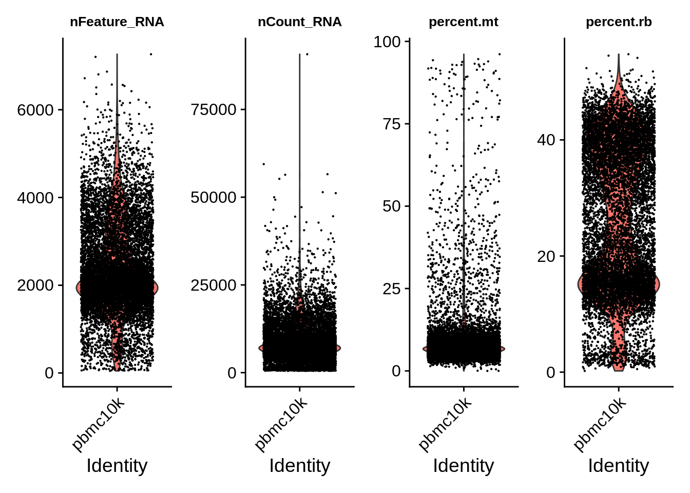
Let’s plot some of the metadata features against each other and see how they correlate. The number above each plot is a Pearson correlation coefficient.
FeatureScatter(srat, feature1 = "nCount_RNA", feature2 = "percent.mt")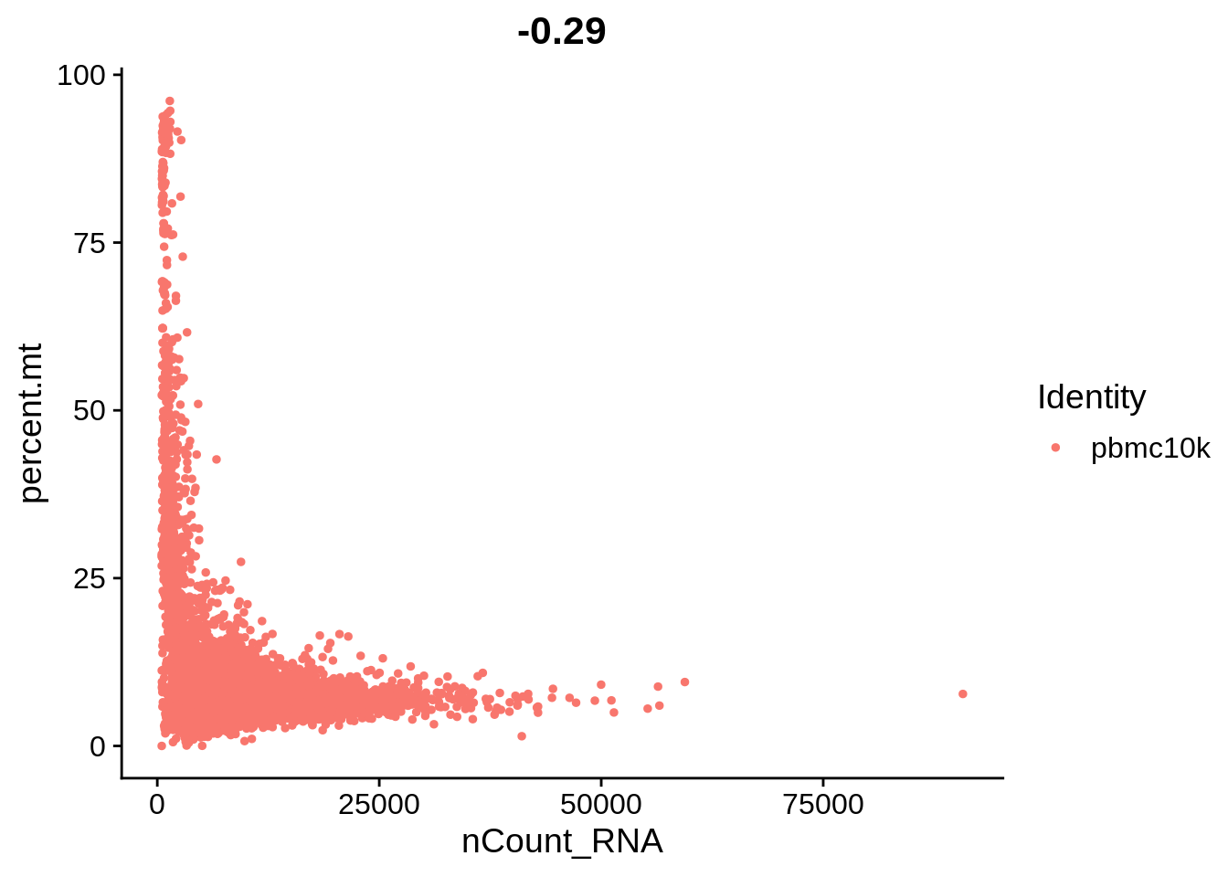
FeatureScatter(srat, feature1 = "nCount_RNA", feature2 = "nFeature_RNA")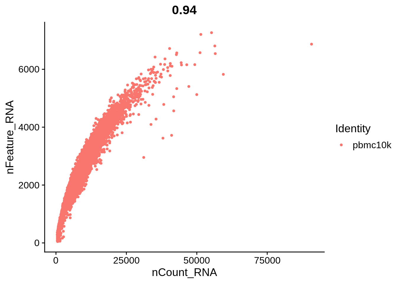
FeatureScatter(srat, feature1 = "nCount_RNA", feature2 = "percent.rb")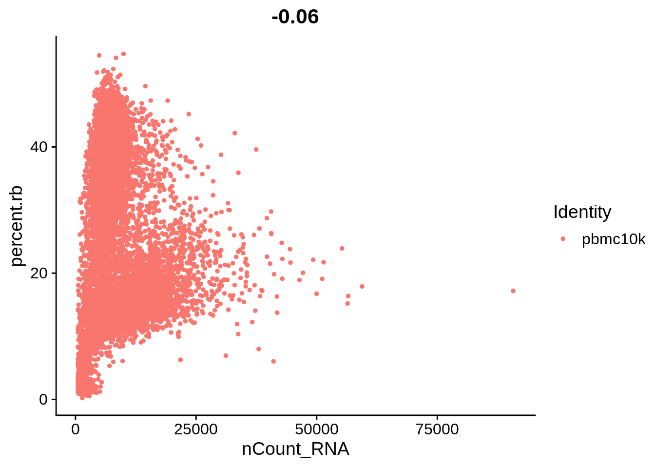
FeatureScatter(srat, feature1 = "percent.rb", feature2 = "percent.mt")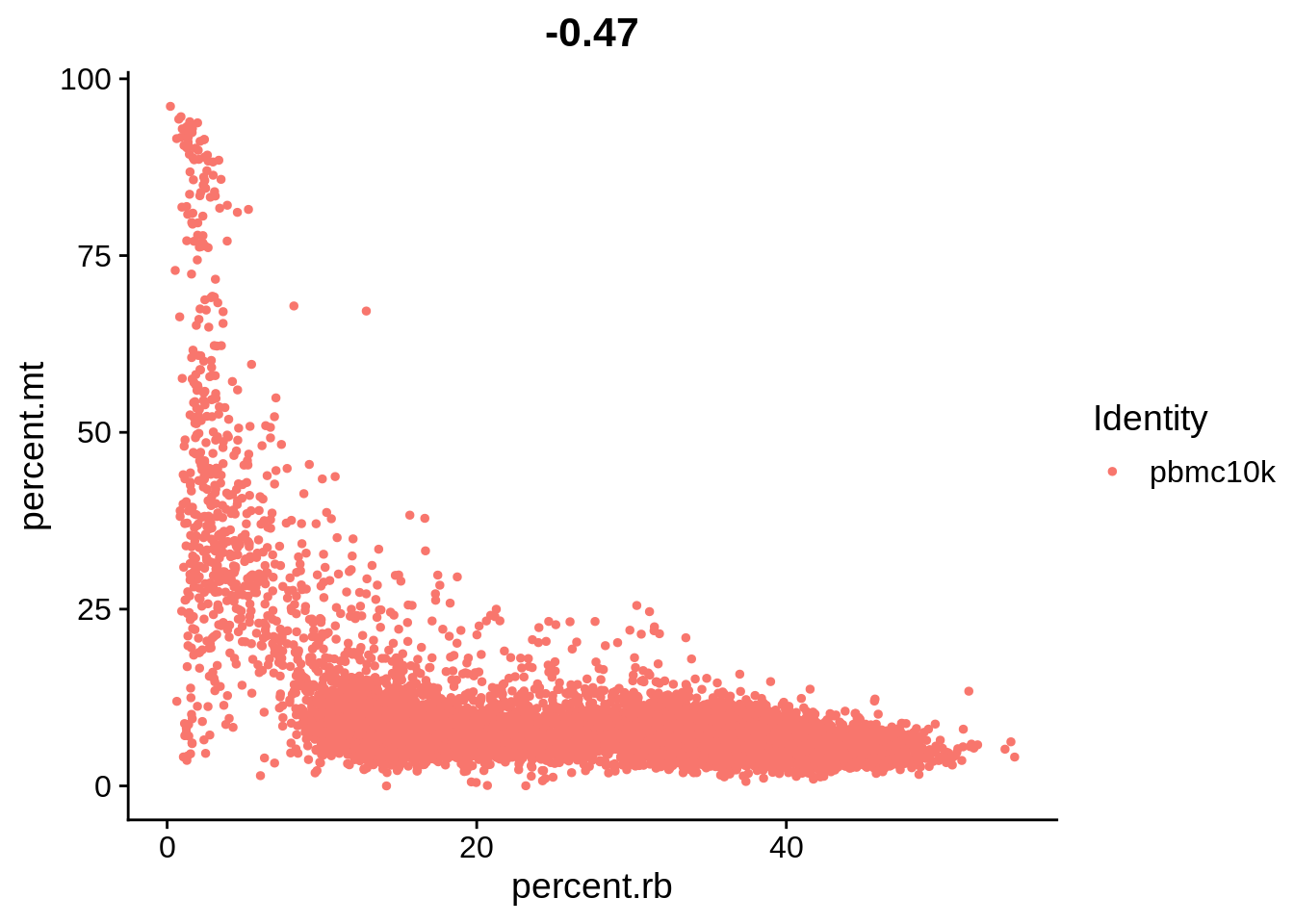
FeatureScatter(srat, feature1 = "nFeature_RNA", feature2 = "Doublet_score")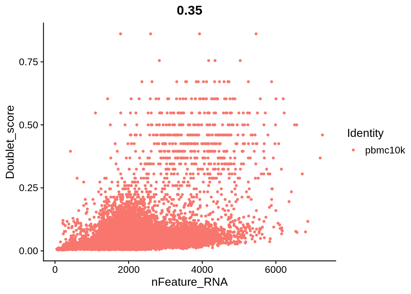
The plots above clearly show that high MT percentage strongly correlates with low UMI counts, and usually is interpreted as dead cells. High ribosomal protein content, however, strongly anti-correlates with MT, and seems to contain biological signal. There’s also a strong correlation between the doublet score and number of expressed genes. Let’s set QC column in metadata and define it in an informative way.
srat[['QC']] <- ifelse(srat@meta.data$Is_doublet == 'True','Doublet','Pass')
srat[['QC']] <- ifelse(srat@meta.data$nFeature_RNA < 500 & srat@meta.data$QC == 'Pass','Low_nFeature',srat@meta.data$QC)
srat[['QC']] <- ifelse(srat@meta.data$nFeature_RNA < 500 & srat@meta.data$QC != 'Pass' & srat@meta.data$QC != 'Low_nFeature',paste('Low_nFeature',srat@meta.data$QC,sep = ','),srat@meta.data$QC)
srat[['QC']] <- ifelse(srat@meta.data$percent.mt > 15 & srat@meta.data$QC == 'Pass','High_MT',srat@meta.data$QC)
srat[['QC']] <- ifelse(srat@meta.data$nFeature_RNA < 500 & srat@meta.data$QC != 'Pass' & srat@meta.data$QC != 'High_MT',paste('High_MT',srat@meta.data$QC,sep = ','),srat@meta.data$QC)
table(srat[['QC']])
## QC
## Doublet High_MT
## 546 548
## High_MT,Low_nFeature High_MT,Low_nFeature,Doublet
## 275 1
## Pass
## 8824We can see that doublets don’t often overlap with cell with low number of detected genes; at the same time, the latter often co-insides with high mitochondrial content. Let’s plot metadata only for cells that pass tentative QC:
VlnPlot(subset(srat, subset = QC == 'Pass'),
        features = c("nFeature_RNA", "nCount_RNA", "percent.mt","percent.rb"), ncol = 4, pt.size = 0.1) &
  theme(plot.title = element_text(size=10))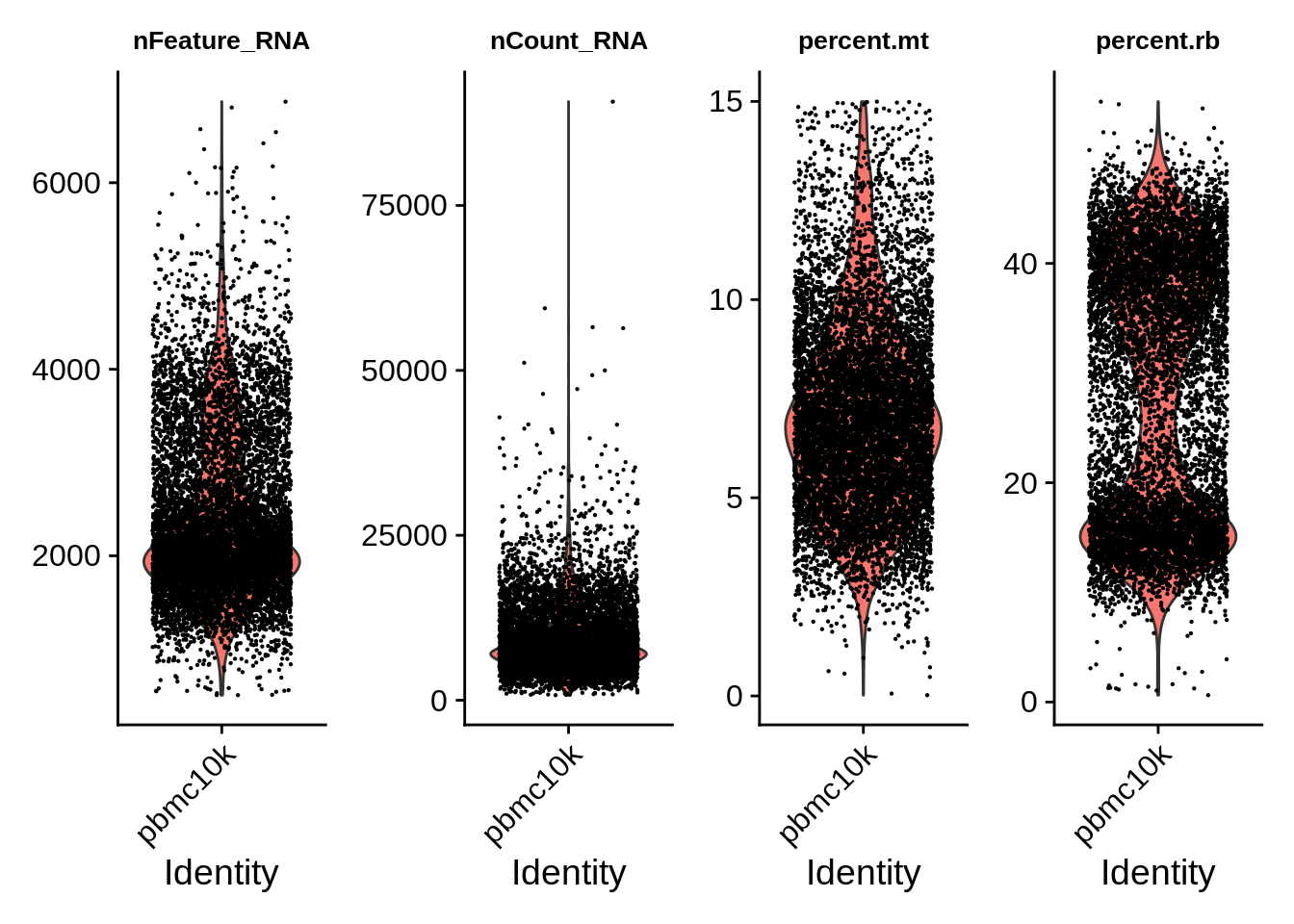
8.2 Normalization and dimensionality reduction
In order to do further analysis, we need to normalize the data to account for sequencing depth. Conventional way is to scale it to 10,000 (as if all cells have 10k UMIs overall), and log2-transform the obtained values. Normalized data are stored in srat[['RNA']]@data of the ‘RNA’ assay.
srat <- NormalizeData(srat)Next step discovers the most variable features (genes) - these are usually most interesting for downstream analysis.
srat <- FindVariableFeatures(srat, selection.method = "vst", nfeatures = 2000)Identify the 10 most highly variable genes:
top10 <- head(VariableFeatures(srat), 10)
top10
## [1] "PTGDS" "IGLC3" "PPBP" "CXCL10" "GZMB" "GP1BB" "JCHAIN" "FCER1A"
## [9] "IGKC" "MZB1"Plot variable features with and without labels:
plot1 <- VariableFeaturePlot(srat)
LabelPoints(plot = plot1, points = top10, repel = TRUE, xnudge = 0, ynudge = 0)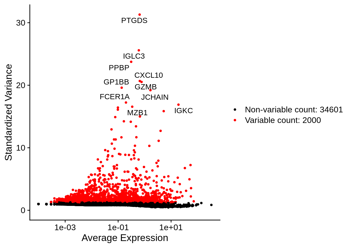
ScaleData converts normalized gene expression to Z-score (values centered at 0 and with variance of 1). It’s stored in srat[['RNA']]@scale.data and used in following PCA. Default is to run scaling only on variable genes.
all.genes <- rownames(srat)
srat <- ScaleData(srat, features = all.genes)
## Centering and scaling data matrixWe can now do PCA, which is a common way of linear dimensionality reduction. By default we use 2000 most variable genes.
srat <- RunPCA(srat, features = VariableFeatures(object = srat))## PC_ 1
## Positive: FCN1, CST3, LYZ, FGL2, IFI30, MNDA, CTSS, TYMP, TYROBP, SERPINA1
## TMEM176B, CYBB, S100A9, PSAP, NCF2, LST1, SPI1, AIF1, IGSF6, CD68
## CSTA, GRN, TNFSF13B, CFD, S100A8, MPEG1, MS4A6A, FCER1G, CFP, DUSP6
## Negative: LTB, IL32, TRAC, TRBC2, IL7R, CD7, LIME1, ARL4C, CD27, PRKCQ-AS1
## CCR7, FCMR, CD247, LEF1, CD69, TRBC1, GZMM, MAL, TRABD2A, BCL2
## SYNE2, ISG20, CTSW, IKZF3, ITM2A, RORA, AQP3, TRAT1, CD8B, KLRK1
## PC_ 2
## Positive: IGHM, MS4A1, CD79A, BANK1, SPIB, NIBAN3, BCL11A, IGKC, CD79B, LINC00926
## TCF4, RALGPS2, AFF3, TNFRSF13C, IGHD, HLA-DQA1, TSPAN13, BLNK, CD22, PAX5
## BLK, COBLL1, VPREB3, FCER2, JCHAIN, FCRLA, GNG7, HLA-DOB, TCL1A, LINC02397
## Negative: IL32, TRAC, CD7, IL7R, CD247, GZMM, ANXA1, CTSW, S100A4, PRKCQ-AS1
## TRBC1, S100A10, ITGB2, LEF1, KLRK1, RORA, GZMA, S100A6, NEAT1, MAL
## CST7, NKG7, ID2, TRBC2, ARL4C, MT2A, SAMD3, PRF1, LIME1, TRAT1
## PC_ 3
## Positive: GZMB, CLIC3, C12orf75, LILRA4, NKG7, CLEC4C, SERPINF1, CST7, GZMA, GNLY
## SCT, LRRC26, DNASE1L3, PRF1, TPM2, KLRD1, FGFBP2, CTSC, PACSIN1, IL3RA
## HOPX, CCL5, PLD4, LINC00996, GZMH, CCL4, MAP1A, SMPD3, TNFRSF21, PTCRA
## Negative: MS4A1, CD79A, LINC00926, BANK1, TNFRSF13C, IGHD, PAX5, RALGPS2, VPREB3, CD22
## FCER2, CD79B, HLA-DOB, FCRL1, P2RX5, CD24, ARHGAP24, ADAM28, CCR7, SWAP70
## FCRLA, LINC02397, CD19, IGHM, CD40, PKIG, FCRL2, BASP1, POU2AF1, BLK
## PC_ 4
## Positive: NKG7, GNLY, CST7, PRF1, KLRD1, GZMA, FGFBP2, HOPX, CCL4, FCGR3A
## KLRF1, GZMH, CCL5, SPON2, CD160, ADGRG1, PTGDR, LAIR2, TRDC, RHOC
## IFITM2, ABI3, MATK, TBX21, IL2RB, XCL2, PRSS23, FCRL6, CTSW, S1PR5
## Negative: LILRA4, SERPINF1, CLEC4C, SCT, LRRC26, DNASE1L3, TPM2, MAP1A, TNFRSF21, PACSIN1
## LINC00996, SCN9A, PTCRA, EPHB1, ITM2C, SMIM5, LAMP5, DERL3, CIB2, APP
## IL3RA, SMPD3, PLEKHD1, SCAMP5, PLD4, ZFAT, PPM1J, GAS6, LGMN, TLR9
## PC_ 5
## Positive: S100A12, VCAN, ITGAM, CES1, S100A8, CYP1B1, PADI4, MGST1, MEGF9, MCEMP1
## QPCT, GNLY, CD14, RNASE2, CSF3R, RBP7, NKG7, KLRD1, VNN2, CLEC4E
## CRISPLD2, THBS1, PRF1, CST7, CKAP4, BST1, CTSD, CR1, FGFBP2, PGD
## Negative: CDKN1C, HES4, CTSL, BATF3, TCF7L2, SIGLEC10, CSF1R, CKB, MS4A7, CALML4
## FCGR3A, CASP5, RRAS, AC064805.1, MS4A4A, NEURL1, AC104809.2, IFITM3, MTSS1, SMIM25
## CAMK1, GPBAR1, ABI3, HMOX1, ZNF703, FAM110A, RHOC, CXCL16, CALHM6, RNASET2Prinicpal component “loadings” should match markers of distinct populations for well behaved datasets. Note that you can change many plot parameters using ggplot2 features - passing them with & operator.
VizDimLoadings(srat, dims = 1:9, reduction = "pca") &
  theme(axis.text=element_text(size=5), axis.title=element_text(size=8,face="bold"))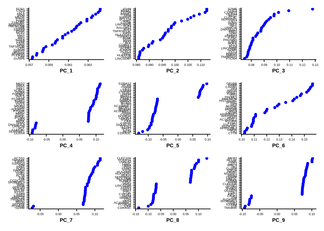
Alternatively, one can do heatmap of each principal component or several PCs at once:
DimHeatmap(srat, dims = 1:6, nfeatures = 20, cells = 500, balanced = T)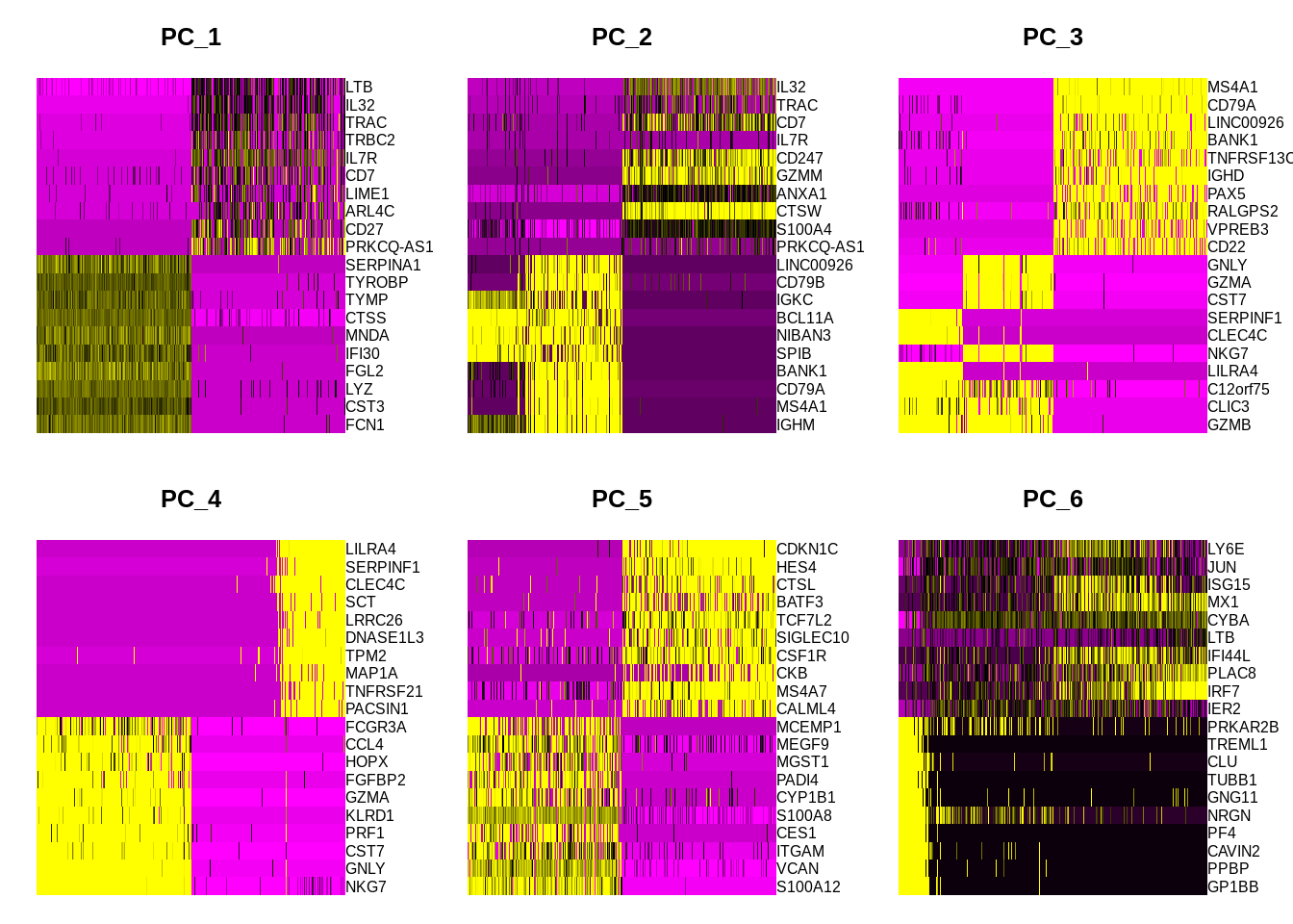
DimPlot is used to visualize all reduced representations (PCA, tSNE, UMAP, etc). Identity is still set to “orig.ident.” DimPlot has built-in hiearachy of dimensionality reductions it tries to plot: first, it looks for UMAP, then (if not available) tSNE, then PCA.
DimPlot(srat, reduction = "pca")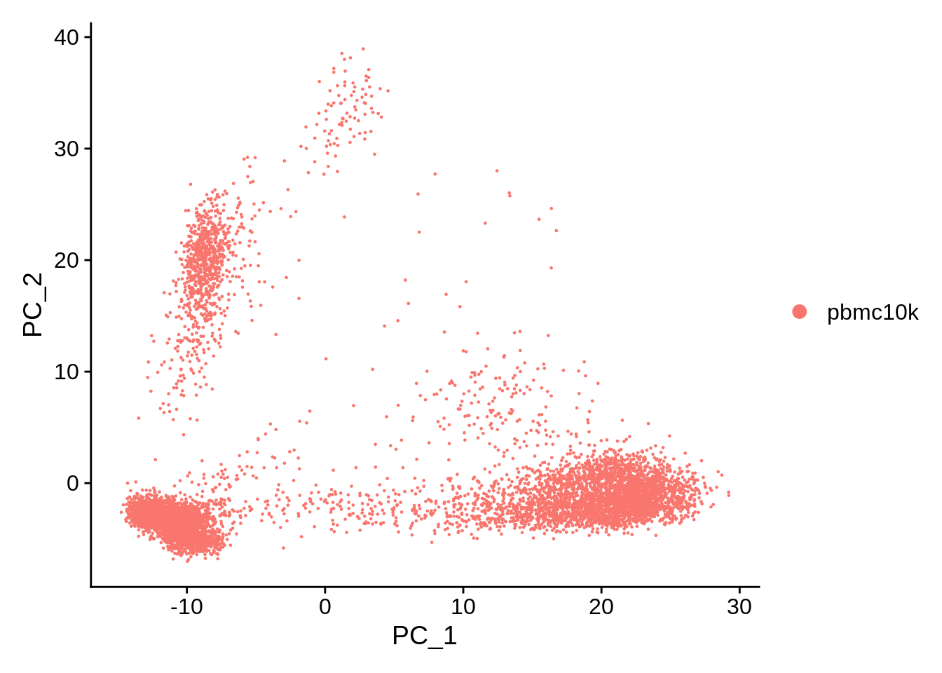
It’s often good to find how many PCs can be used without much information loss. In our case a big drop happens at 10, so seems like a good initial choice:
ElbowPlot(srat)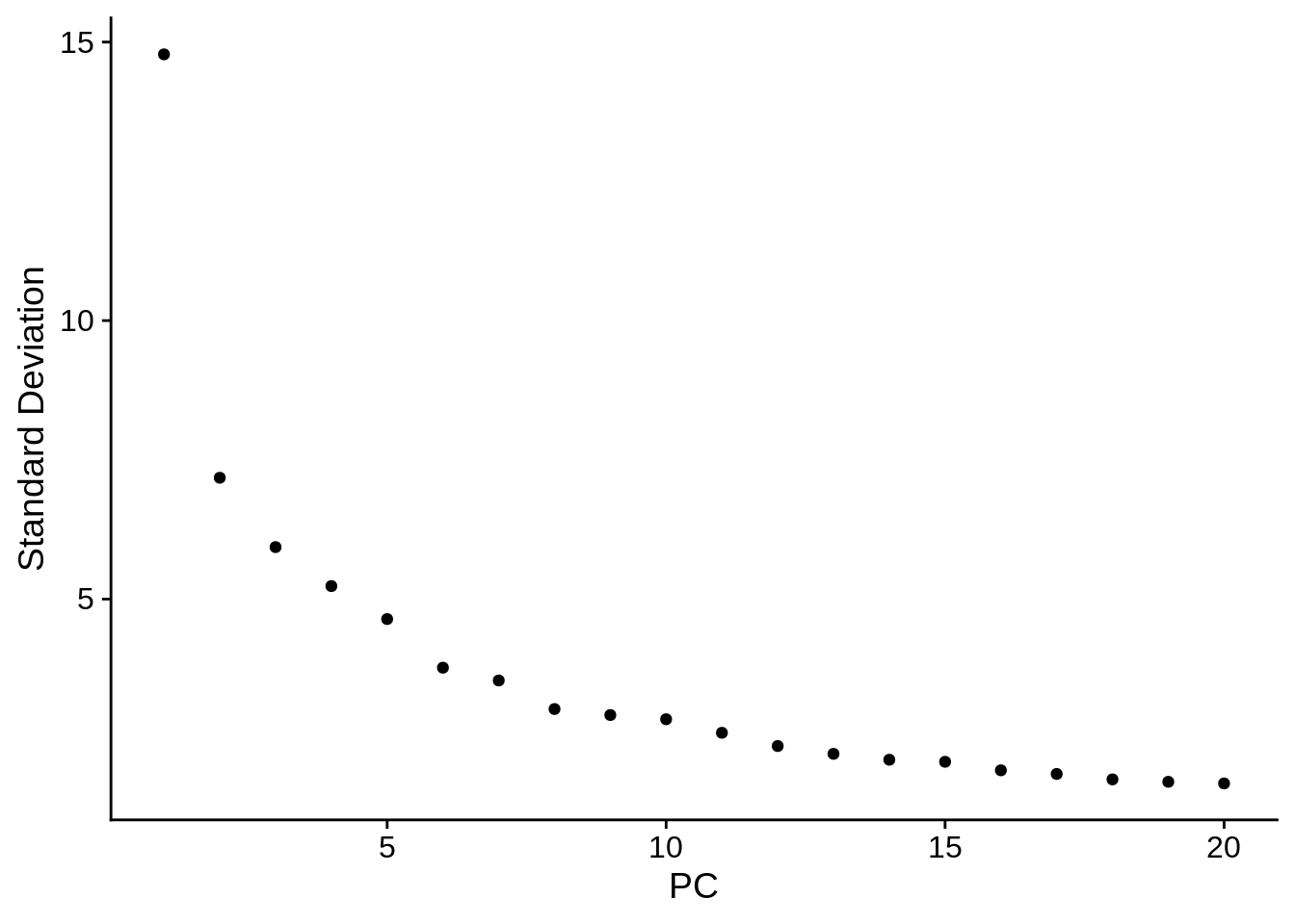
We can now do clustering. Higher resolution leads to more clusters (default is 0.8). It would be very important to find the correct cluster resolution in the future, since cell type markers depends on cluster definition.
srat <- FindNeighbors(srat, dims = 1:10)## Computing nearest neighbor graph## Computing SNNsrat <- FindClusters(srat, resolution = 0.5)## Modularity Optimizer version 1.3.0 by Ludo Waltman and Nees Jan van Eck
##
## Number of nodes: 10194
## Number of edges: 337796
##
## Running Louvain algorithm...
## Maximum modularity in 10 random starts: 0.9082
## Number of communities: 13
## Elapsed time: 2 secondsFor visualization purposes, we also need to generate UMAP reduced dimensionality representation:
srat <- RunUMAP(srat, dims = 1:10, verbose = F)## Warning: The default method for RunUMAP has changed from calling Python UMAP via reticulate to the R-native UWOT using the cosine metric
## To use Python UMAP via reticulate, set umap.method to 'umap-learn' and metric to 'correlation'
## This message will be shown once per sessionOnce clustering is done, active identity is reset to clusters (“seurat_clusters” in metadata). Let’s look at cluster sizes.
table(srat@meta.data$seurat_clusters)##
## 0 1 2 3 4 5 6 7 8 9 10 11 12
## 2854 1671 1163 1079 851 774 426 402 381 245 178 134 36DimPlot uses UMAP by default, with Seurat clusters as identity:
DimPlot(srat,label.size = 4,repel = T,label = T)
In order to control for clustering resolution and other possible artifacts, we will take a close look at two minor cell populations: 1) dendritic cells (DCs), 2) platelets, aka thrombocytes. Let’s visualise two markers for each of this cell type: LILRA4 and TPM2 for DCs, and PPBP and GP1BB for platelets.
FeaturePlot(srat, features = c("LILRA4", "TPM2", "PPBP", "GP1BB"))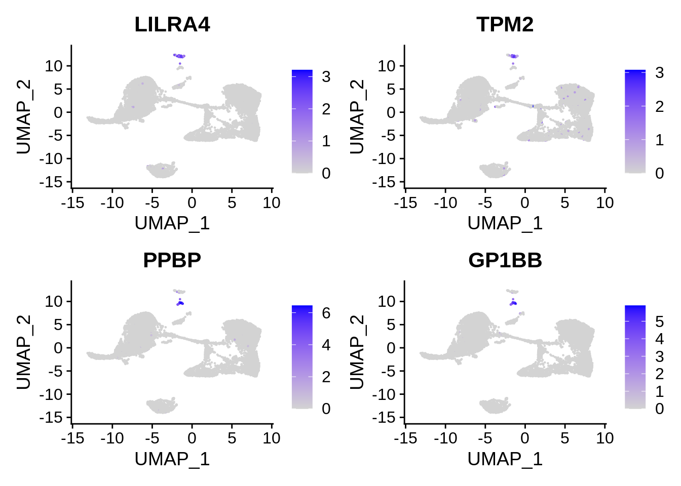
Let’s visualize other confounders:
FeaturePlot(srat, features = "Doublet_score") & theme(plot.title = element_text(size=10))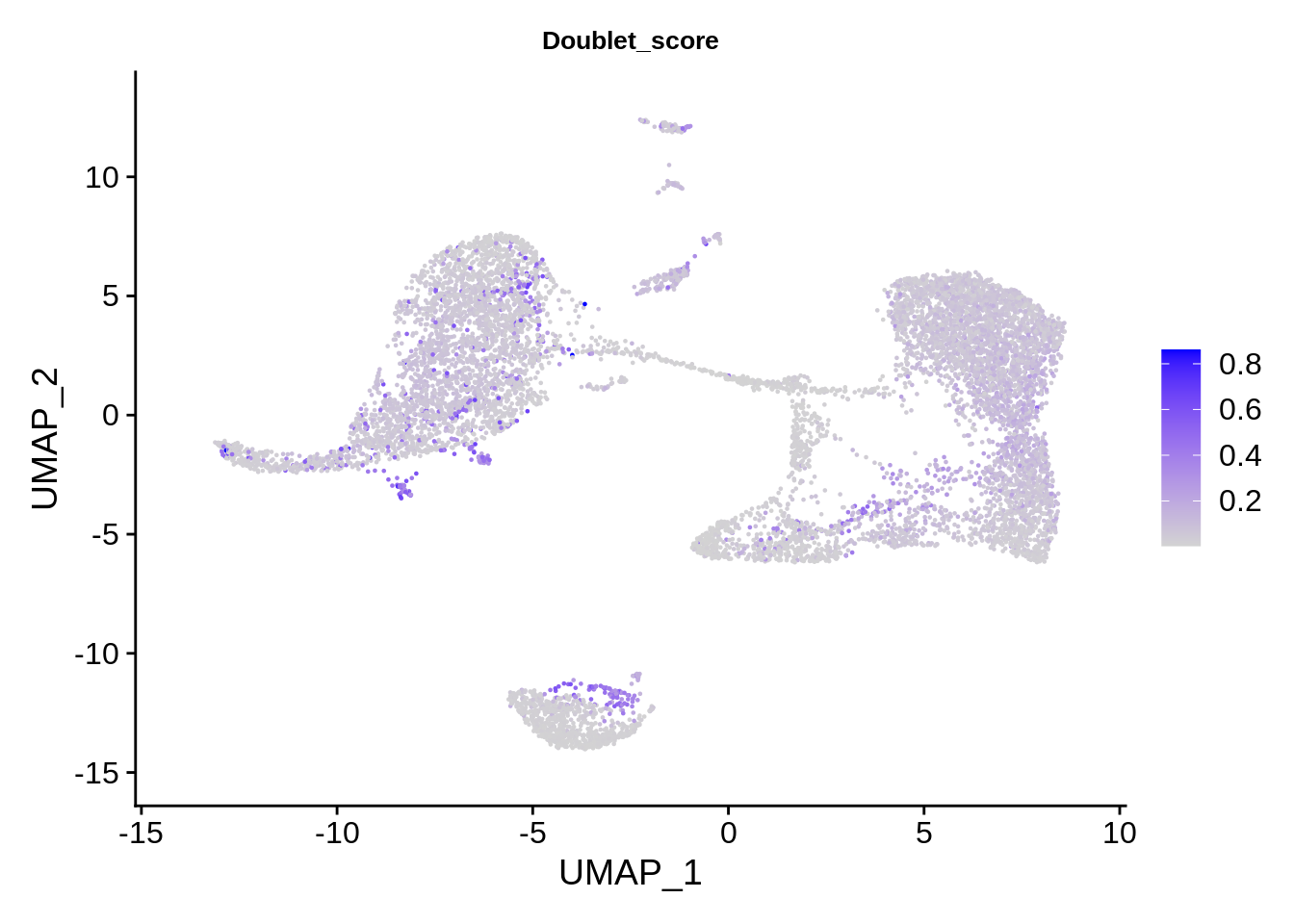
FeaturePlot(srat, features = "percent.mt") & theme(plot.title = element_text(size=10))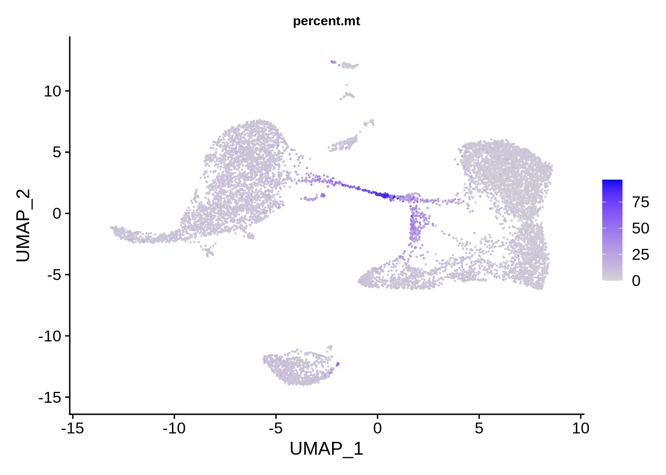
FeaturePlot(srat, features = "nFeature_RNA") & theme(plot.title = element_text(size=10))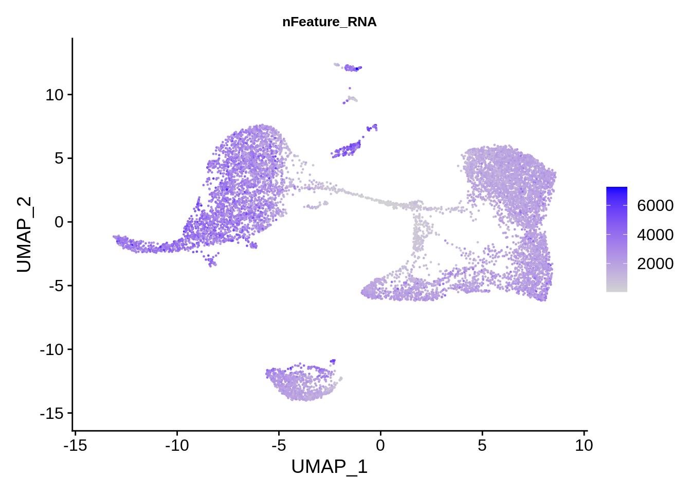
Let’s remove the cells that did not pass QC and compare plots. We can now see much more defined clusters. Our filtered dataset now contains 8824 cells - so approximately 12% of cells were removed for various reasons.
DimPlot(srat,label.size = 4,repel = T,label = T)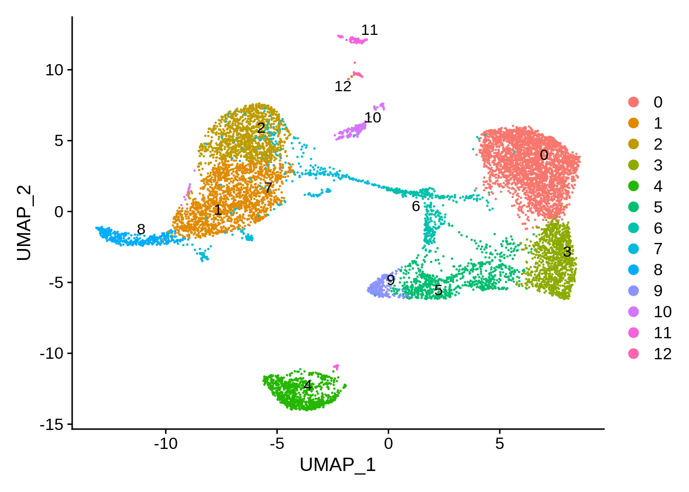
srat <- subset(srat, subset = QC == 'Pass')
DimPlot(srat,label.size = 4,repel = T,label = T)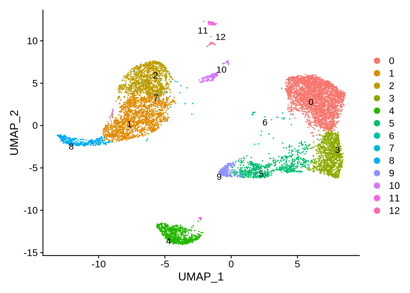
Finally, let’s calculate cell cycle scores, as described here. This has to be done after normalization and scaling. Seurat has a built-in list, cc.genes (older) and cc.genes.updated.2019 (newer), that defines genes involved in cell cycle. For CellRanger reference GRCh38 2.0.0 and above, use cc.genes.updated.2019 (three genes were renamed: MLF1IP, FAM64A and HN1 became CENPU, PICALM and JPT). For mouse cell cycle genes you can use the solution detailed here.
cc.genes.updated.2019## $s.genes
## [1] "MCM5" "PCNA" "TYMS" "FEN1" "MCM7" "MCM4"
## [7] "RRM1" "UNG" "GINS2" "MCM6" "CDCA7" "DTL"
## [13] "PRIM1" "UHRF1" "CENPU" "HELLS" "RFC2" "POLR1B"
## [19] "NASP" "RAD51AP1" "GMNN" "WDR76" "SLBP" "CCNE2"
## [25] "UBR7" "POLD3" "MSH2" "ATAD2" "RAD51" "RRM2"
## [31] "CDC45" "CDC6" "EXO1" "TIPIN" "DSCC1" "BLM"
## [37] "CASP8AP2" "USP1" "CLSPN" "POLA1" "CHAF1B" "MRPL36"
## [43] "E2F8"
##
## $g2m.genes
## [1] "HMGB2" "CDK1" "NUSAP1" "UBE2C" "BIRC5" "TPX2" "TOP2A"
## [8] "NDC80" "CKS2" "NUF2" "CKS1B" "MKI67" "TMPO" "CENPF"
## [15] "TACC3" "PIMREG" "SMC4" "CCNB2" "CKAP2L" "CKAP2" "AURKB"
## [22] "BUB1" "KIF11" "ANP32E" "TUBB4B" "GTSE1" "KIF20B" "HJURP"
## [29] "CDCA3" "JPT1" "CDC20" "TTK" "CDC25C" "KIF2C" "RANGAP1"
## [36] "NCAPD2" "DLGAP5" "CDCA2" "CDCA8" "ECT2" "KIF23" "HMMR"
## [43] "AURKA" "PSRC1" "ANLN" "LBR" "CKAP5" "CENPE" "CTCF"
## [50] "NEK2" "G2E3" "GAS2L3" "CBX5" "CENPA"s.genes <- cc.genes.updated.2019$s.genes
g2m.genes <- cc.genes.updated.2019$g2m.genes
srat <- CellCycleScoring(srat, s.features = s.genes, g2m.features = g2m.genes)
table(srat[[]]$Phase)##
## G1 G2M S
## 5431 977 2416Let’s see if we have clusters defined by any of the technical differences. Mitochnondrial genes show certain dependency on cluster, being much lower in clusters 2 and 12.
FeaturePlot(srat,features = "percent.mt",label.size = 4,repel = T,label = T) &
  theme(plot.title = element_text(size=10))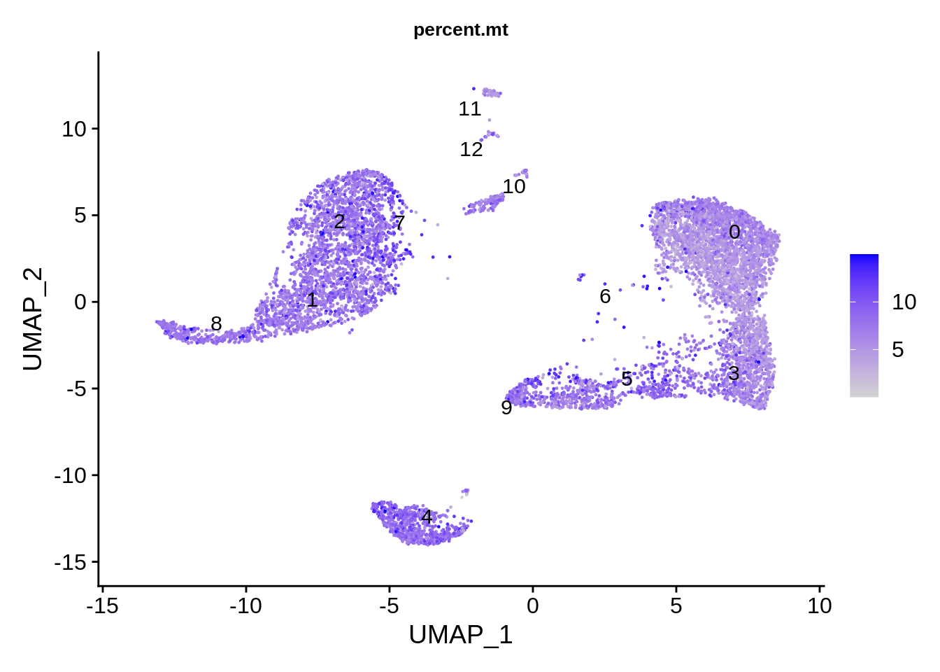
VlnPlot(srat,features = "percent.mt") & theme(plot.title = element_text(size=10))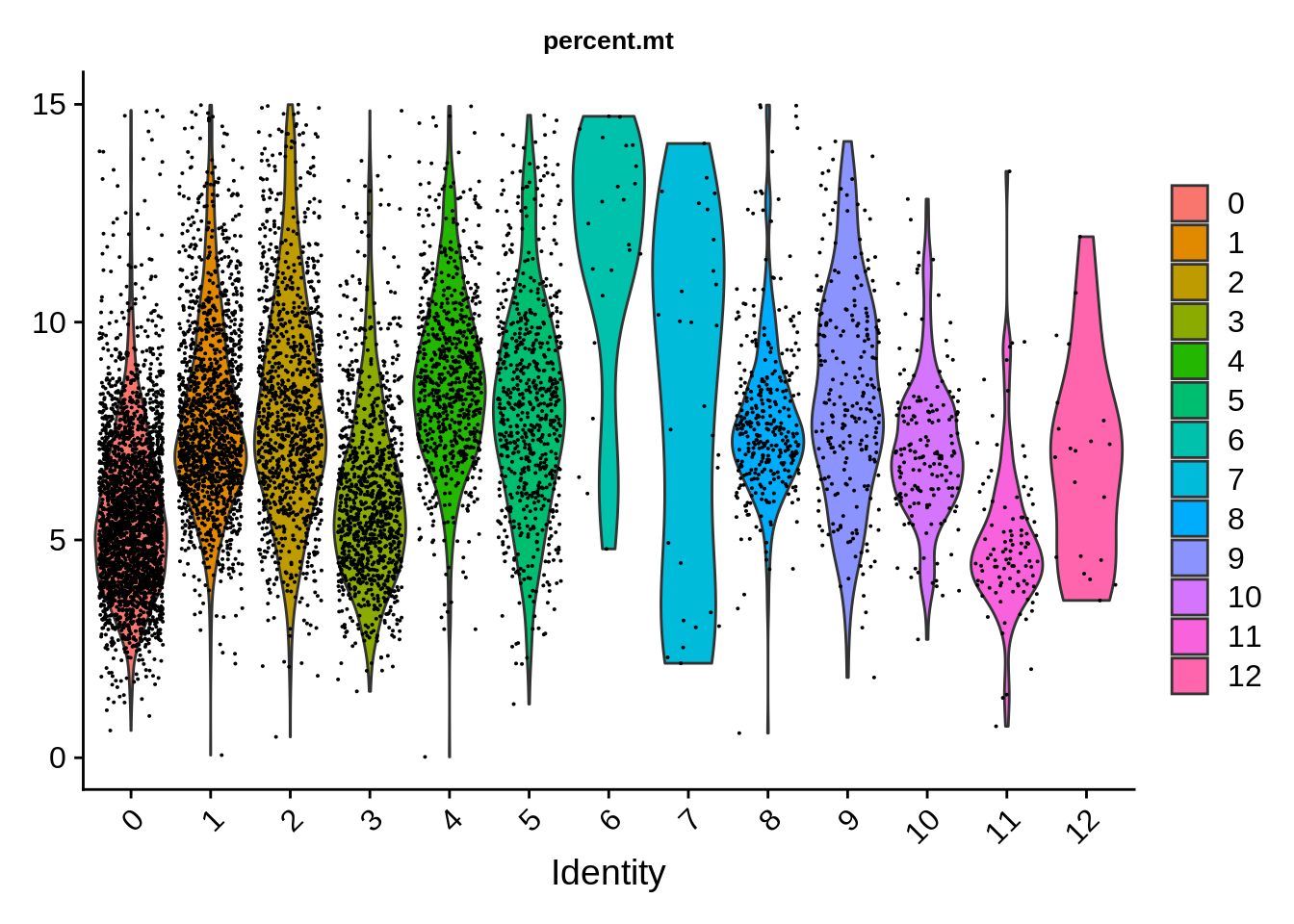
Ribosomal protein genes show very strong dependency on the putative cell type! Some cell clusters seem to have as much as 45%, and some as little as 15%.
FeaturePlot(srat,features = "percent.rb",label.size = 4,repel = T,label = T) & theme(plot.title = element_text(size=10))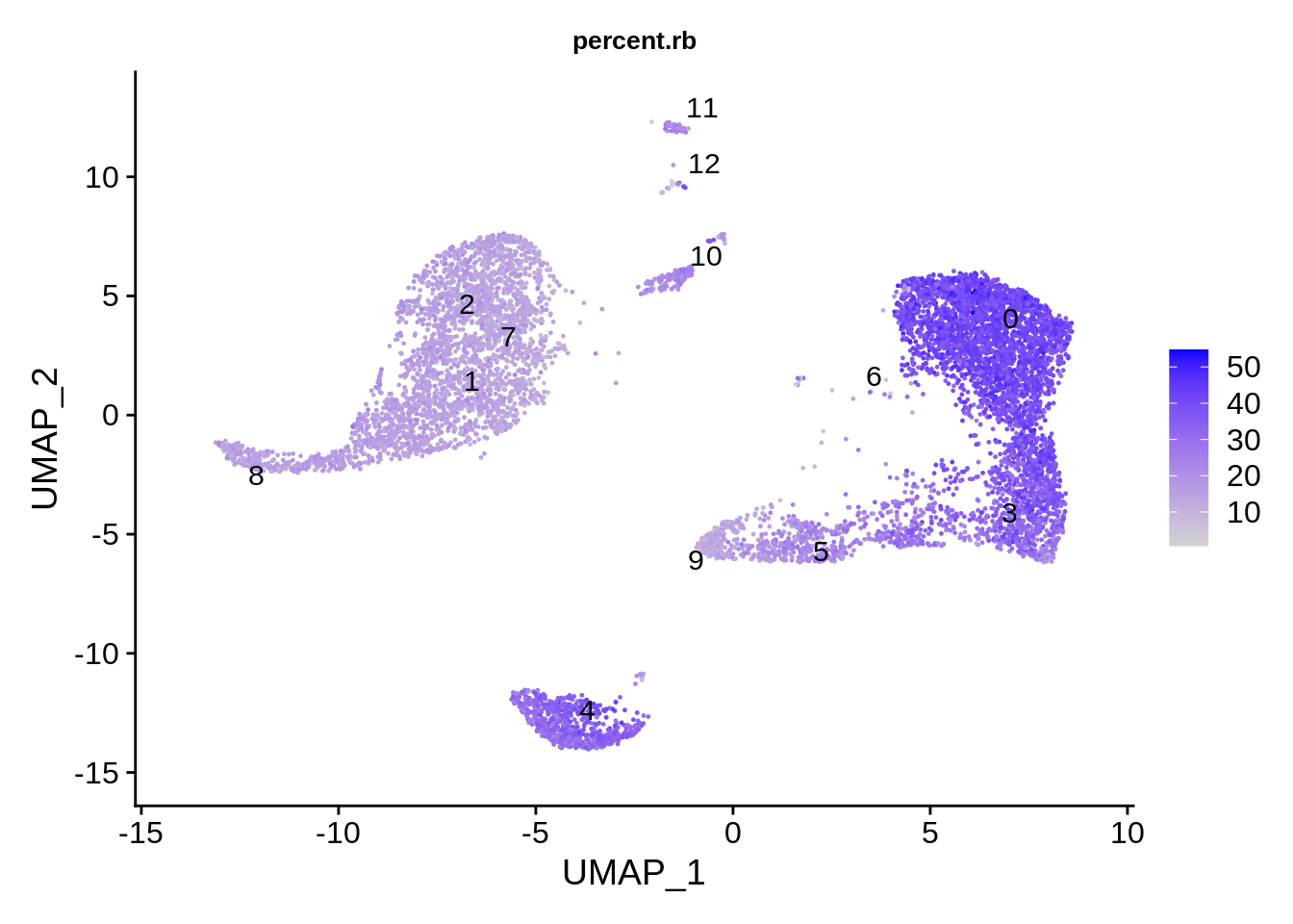
VlnPlot(srat,features = "percent.rb") & theme(plot.title = element_text(size=10))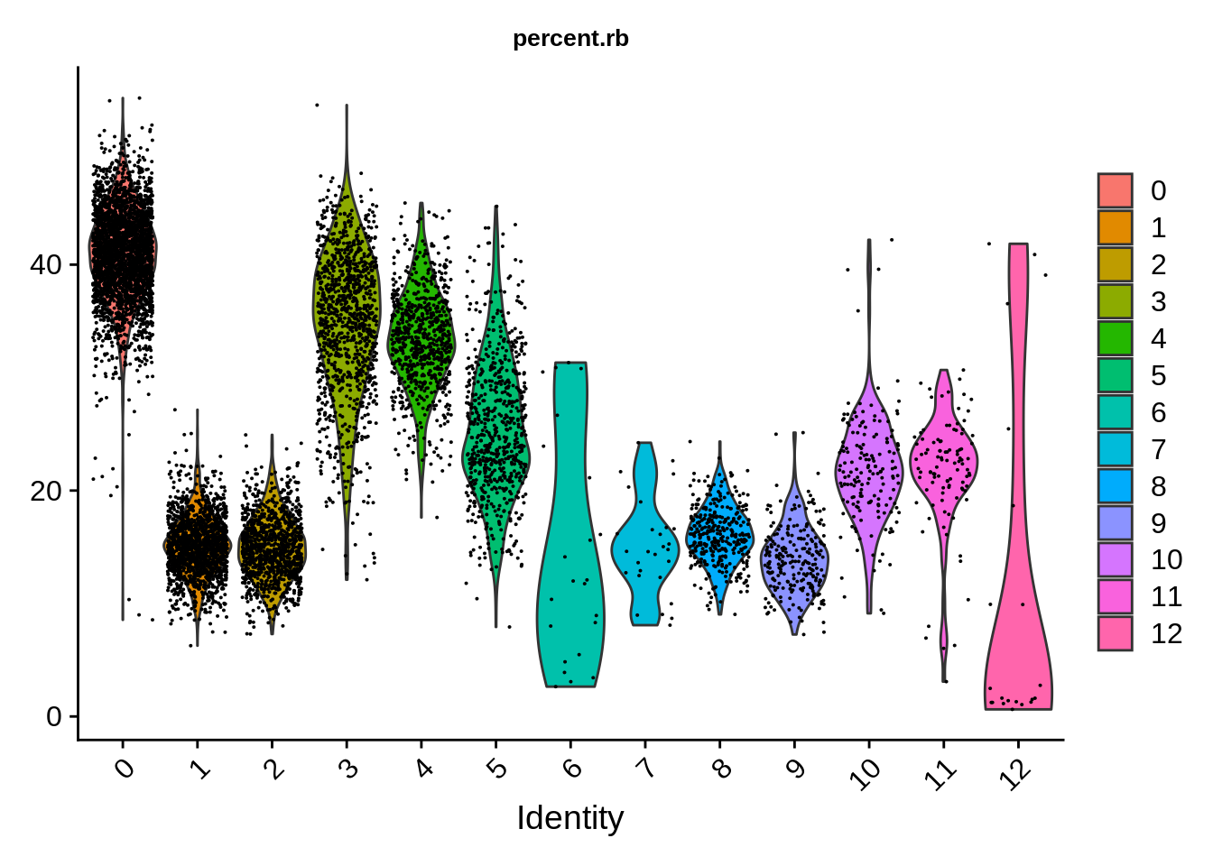
There are also differences in RNA content per cell type. From earlier considerations, clusters 6 and 7 are probably lower quality cells that will disapper when we redo the clustering using the QC-filtered dataset.
VlnPlot(srat,features = c("nCount_RNA","nFeature_RNA")) &
  theme(plot.title = element_text(size=10))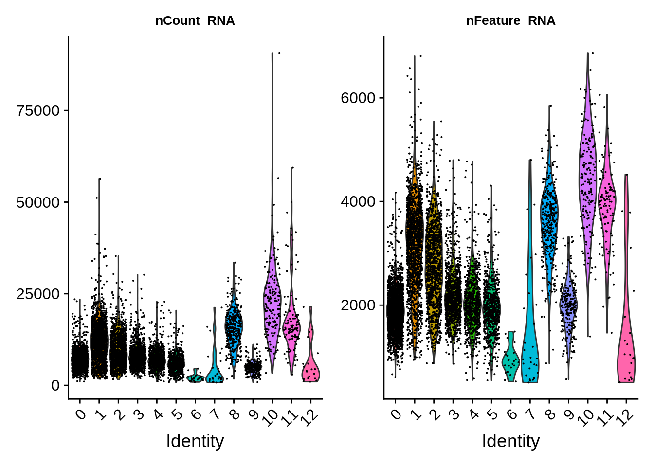
Finally, cell cycle score does not seem to depend on the cell type much - however, there are dramatic outliers in each group.
FeaturePlot(srat,features = c("S.Score","G2M.Score"),label.size = 4,repel = T,label = T) &
  theme(plot.title = element_text(size=10))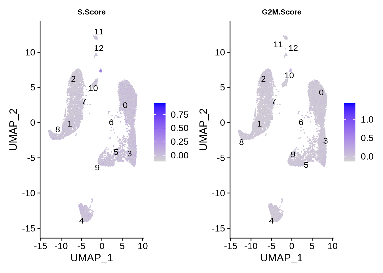
VlnPlot(srat,features = c("S.Score","G2M.Score")) &
  theme(plot.title = element_text(size=10))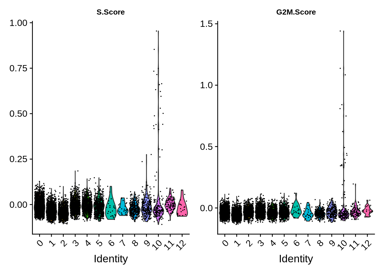
8.3 SCTransform normalization and clustering
Since we have performed extensive QC with doublet and empty cell removal, we can now apply SCTransform normalization, that was shown to be beneficial for finding rare cell populations by improving signal/noise ratio. Single SCTransform command replaces NormalizeData, ScaleData, and FindVariableFeatures. We will also correct for % MT genes and cell cycle scores using vars.to.regress variables; our previous exploration has shown that neither cell cycle score nor MT percentage change very dramatically between clusters, so we will not remove biological signal, but only some unwanted variation.
srat <- SCTransform(srat, method = "glmGamPoi", ncells = 8824,
                    vars.to.regress = c("percent.mt","S.Score","G2M.Score"), verbose = F)
srat
## An object of class Seurat
## 56857 features across 8824 samples within 2 assays
## Active assay: SCT (20256 features, 3000 variable features)
## 1 other assay present: RNA
## 2 dimensional reductions calculated: pca, umapAfter this let’s do standard PCA, UMAP, and clustering. Note that SCT is the active assay now. It is conventional to use more PCs with SCTransform; the exact number can be adjusted depending on your dataset.
srat <- RunPCA(srat, verbose = F)
srat <- RunUMAP(srat, dims = 1:30, verbose = F)
srat <- FindNeighbors(srat, dims = 1:30, verbose = F)
srat <- FindClusters(srat, verbose = F)
table(srat[[]]$seurat_clusters)
##
## 0 1 2 3 4 5 6 7 8 9 10 11 12 13 14 15
## 1766 1554 1214 1066 927 379 328 316 301 268 249 131 107 103 98 17DimPlot(srat, label = T)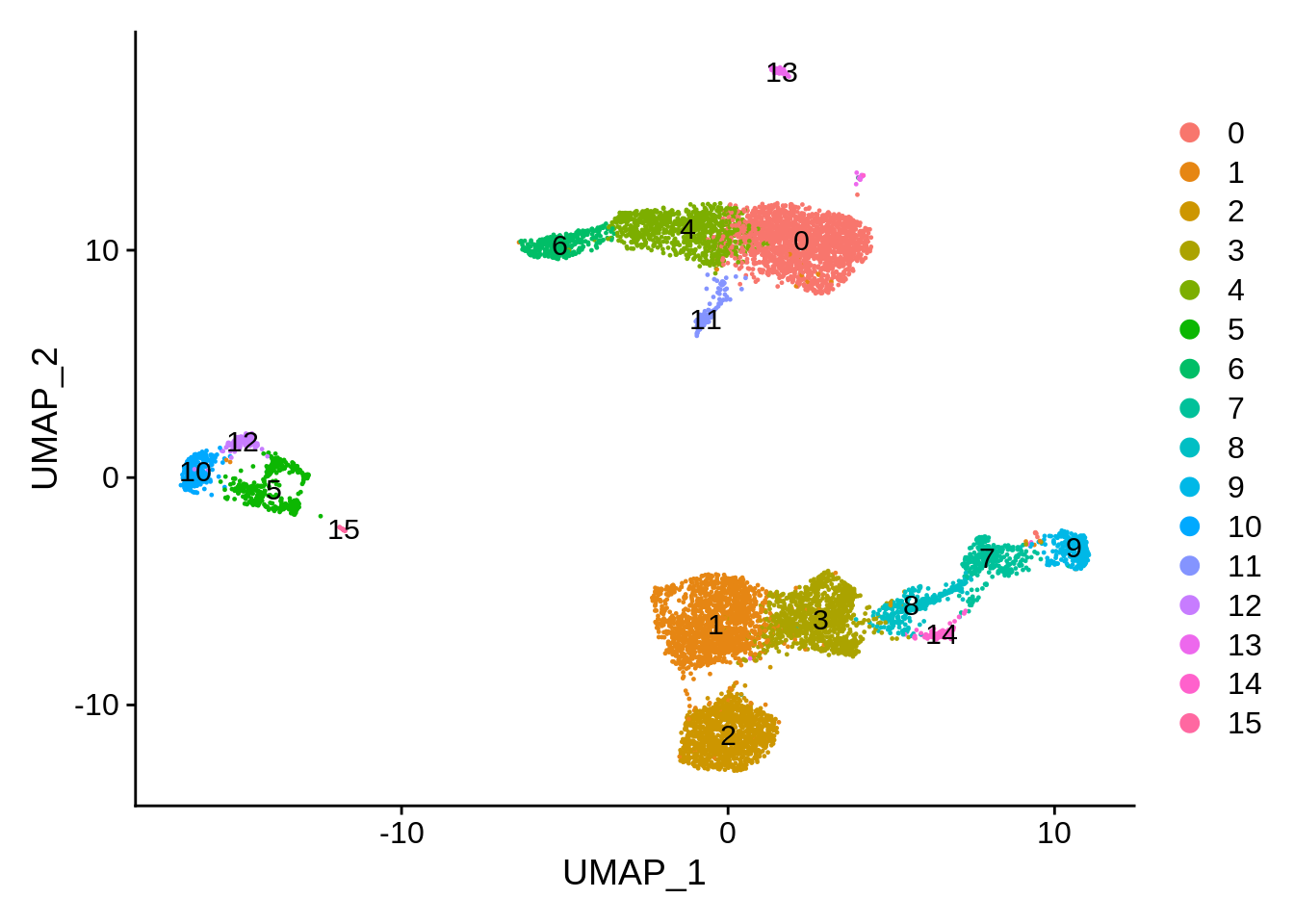
It is very important to define the clusters correctly. Let’s check the markers of smaller cell populations we have mentioned before - namely, platelets and dendritic cells. Let’s also try another color scheme - just to show how it can be done.
FeaturePlot(srat,"PPBP") &
  scale_colour_gradientn(colours = rev(brewer.pal(n = 11, name = "Spectral")))
FeaturePlot(srat,"LILRA4") &
  scale_colour_gradientn(colours = rev(brewer.pal(n = 11, name = "Spectral")))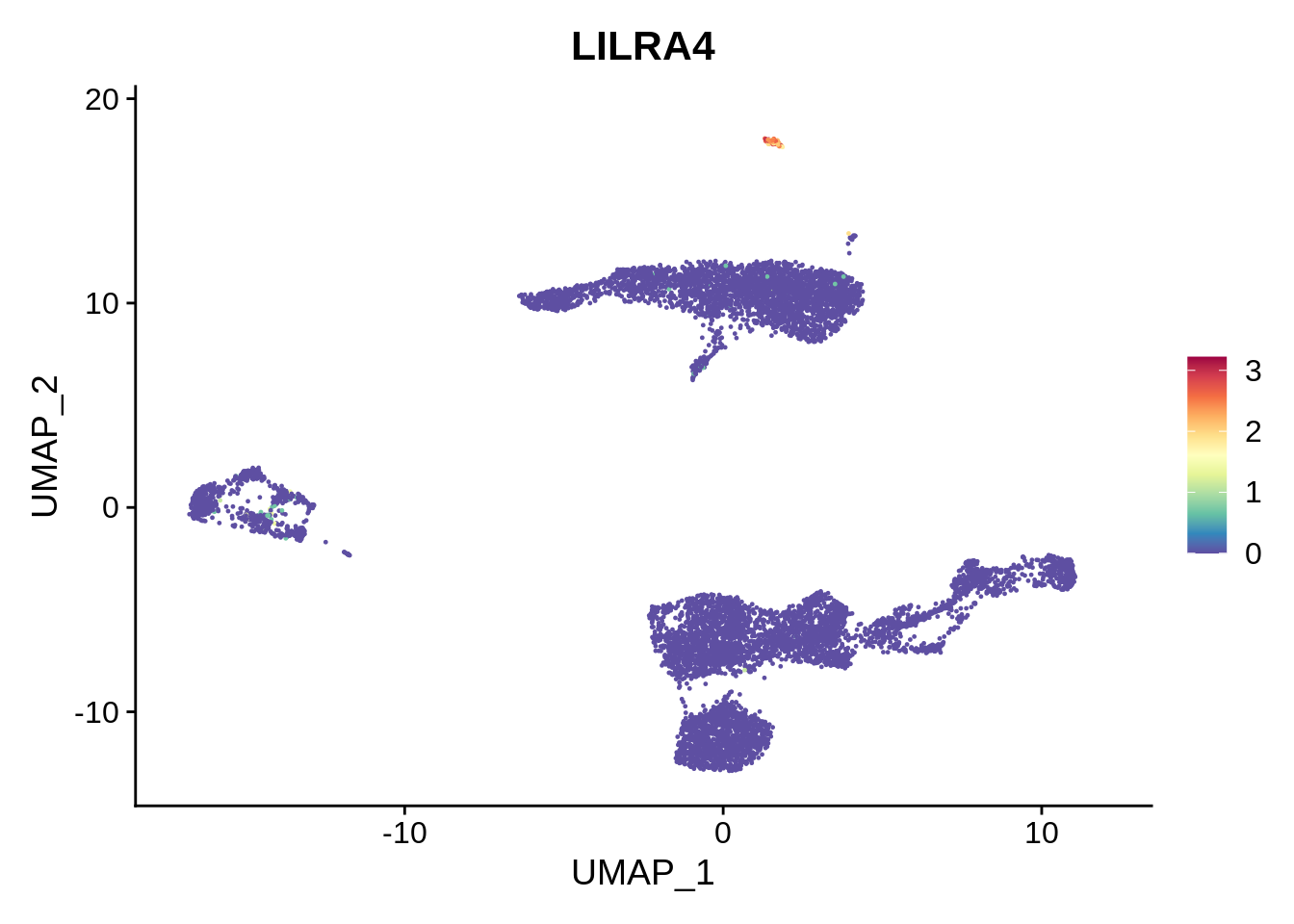
We can see there’s a cluster of platelets located between clusters 6 and 14, that has not been identified. Increasing clustering resolution in FindClusters to 2 would help separate the platelet cluster (try it!), but also generates too many clusters.
If need arises, we can separate some clusters manualy. There are also clustering methods geared towards indentification of rare cell populations. Let’s try using fewer neighbors in the KNN graph, combined with Leiden algorithm (now default in scanpy) and slightly increased resolution:
srat <- FindNeighbors(srat, dims = 1:30, k.param = 15, verbose = F)
srat <- FindClusters(srat, verbose = F, algorithm = 4, resolution = 0.9)table(srat[[]]$seurat_clusters)##
## 1 2 3 4 5 6 7 8 9 10 11 12 13 14 15 16
## 1738 1342 1211 1056 934 380 332 318 315 265 251 211 133 105 104 99
## 17 18
## 17 13DimPlot(srat, label = T)
We already know that cluster 16 corresponds to platelets, and cluster 15 to dendritic cells. Let’s get a very crude idea of what the big cell clusters are.
FeaturePlot(srat,"MS4A1") +
  scale_colour_gradientn(colours = rev(brewer.pal(n = 11, name = "Spectral"))) + ggtitle("MS4A1: B cells")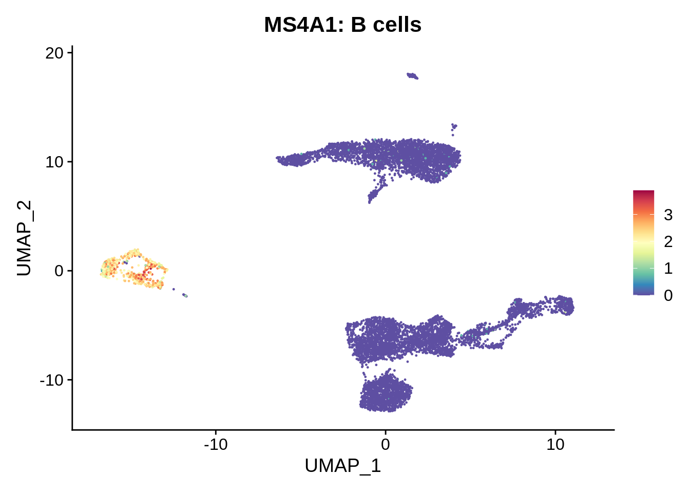
FeaturePlot(srat,"LYZ") +
  scale_colour_gradientn(colours = rev(brewer.pal(n = 11, name = "Spectral"))) + ggtitle("LYZ: monocytes")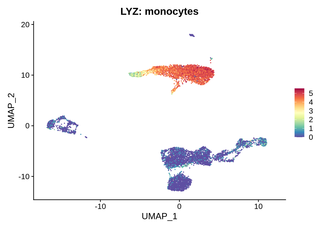
FeaturePlot(srat,"NKG7") +
  scale_colour_gradientn(colours = rev(brewer.pal(n = 11, name = "Spectral"))) + ggtitle("NKG7: natural killers")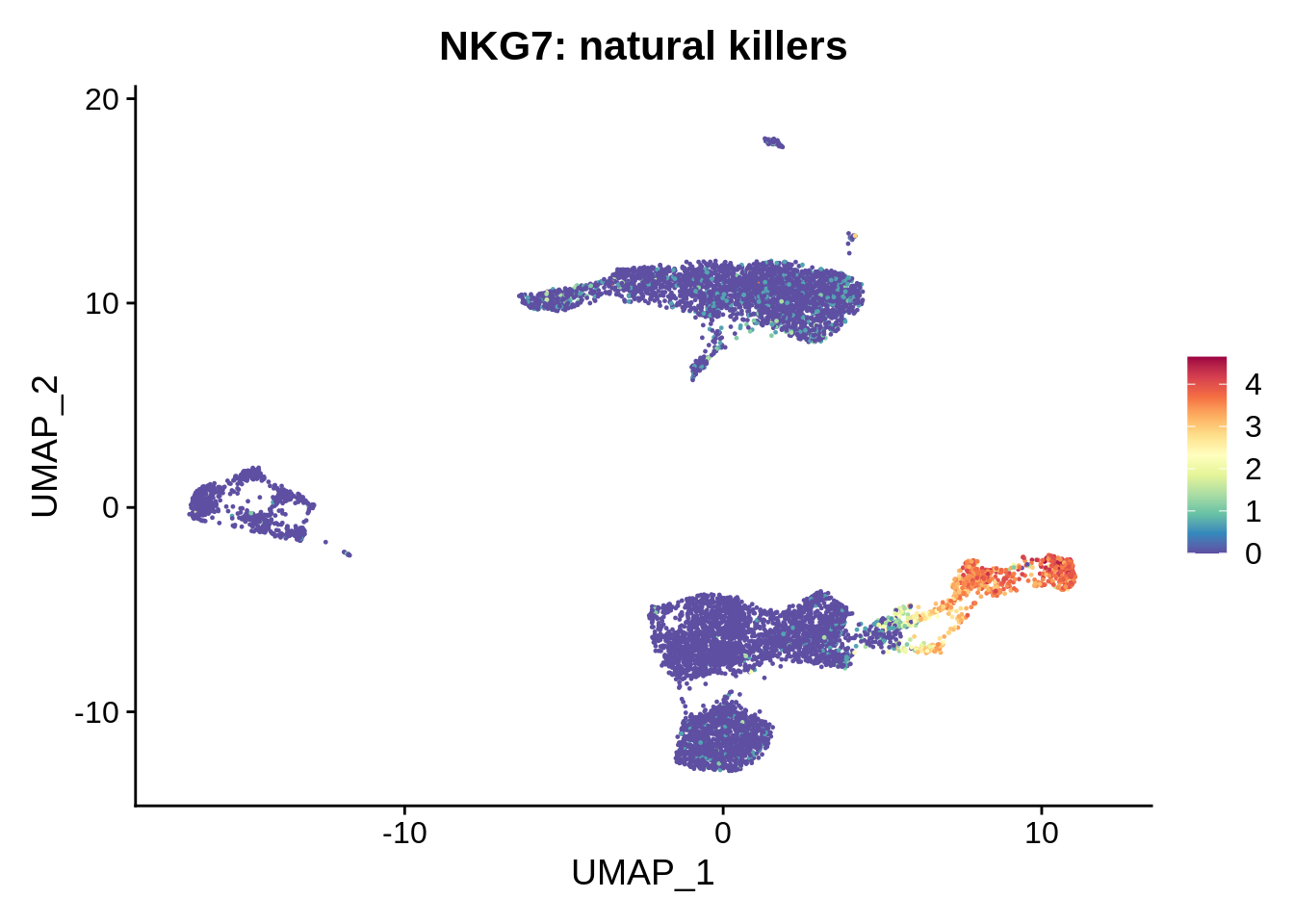
FeaturePlot(srat,"CD8B") +
  scale_colour_gradientn(colours = rev(brewer.pal(n = 11, name = "Spectral"))) + ggtitle("CD8B: CD8 T cells")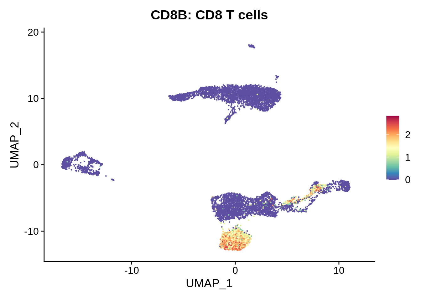
FeaturePlot(srat,"IL7R") +
  scale_colour_gradientn(colours = rev(brewer.pal(n = 11, name = "Spectral"))) + ggtitle("IL7R: CD4 T cells")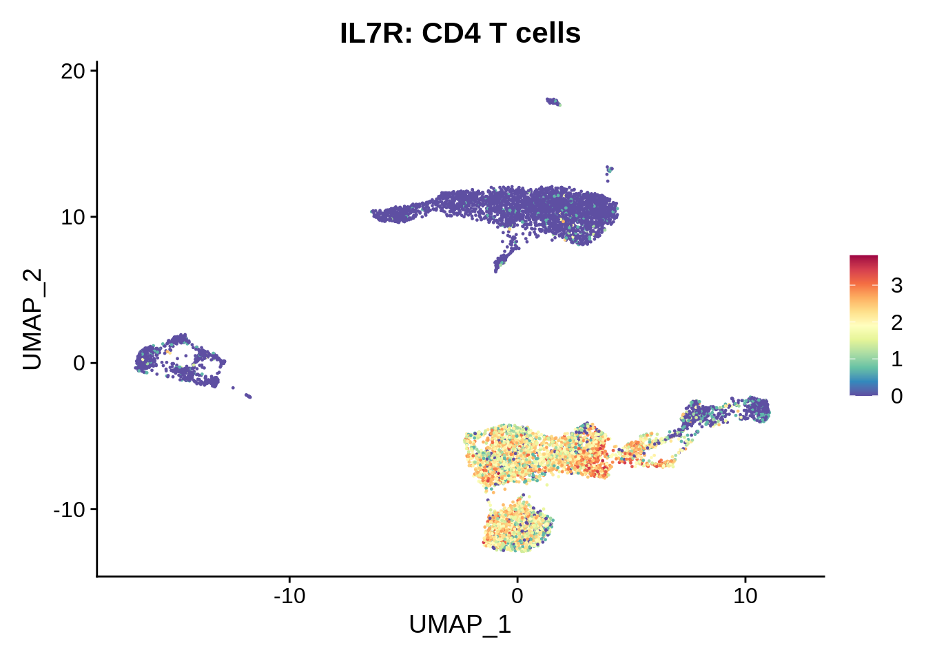
We can see better separation of some subpopulations. These will be further addressed below.
8.4 Differential expression and marker selection
Differential expression allows us to define gene markers specific to each cluster. By definition it is influenced by how clusters are defined, so it’s important to find the correct resolution of your clustering before defining the markers. If some clusters lack any notable markers, adjust the clustering. It is recommended to do differential expression on the RNA assay, and not the SCTransform. Differential expression can be done between two specific clusters, as well as between a cluster and all other cells.
First, let’s set the active assay back to “RNA,” and re-do the normalization and scaling (since we removed a notable fraction of cells that failed QC):
DefaultAssay(srat) <- "RNA"
srat <- NormalizeData(srat)
srat <- FindVariableFeatures(srat, selection.method = "vst", nfeatures = 2000)
all.genes <- rownames(srat)
srat <- ScaleData(srat, features = all.genes)
## Centering and scaling data matrixThe following function allows to find markers for every cluster by comparing it to all remaining cells, while reporting only the positive ones. There are many tests that can be used to define markers, including a very fast and intuitive tf-idf. By default, Wilcoxon Rank Sum test is used. This takes a while - take few minutes to make coffee or a cup of tea! For speed, we have increased the default minimal percentage and log2FC cutoffs; these should be adjusted to suit your dataset!
all.markers <- FindAllMarkers(srat, only.pos = T, min.pct = 0.5, logfc.threshold = 0.5)Let’s take a quick glance at the markers.
dim(all.markers)## [1] 4898 7table(all.markers$cluster)##
## 1 2 3 4 5 6 7 8 9 10 11 12 13 14 15 16 17 18
## 544 131 130 74 530 145 447 183 62 261 154 84 249 152 524 117 224 887top3_markers <- as.data.frame(all.markers %>% group_by(cluster) %>% top_n(n = 3, wt = avg_log2FC))
top3_markers## p_val avg_log2FC pct.1 pct.2 p_val_adj cluster gene
## 1 0.000000e+00 4.5268744 0.997 0.177 0.000000e+00 1 S100A8
## 2 0.000000e+00 4.2834962 0.997 0.200 0.000000e+00 1 S100A9
## 3 0.000000e+00 3.2865113 0.972 0.115 0.000000e+00 1 S100A12
## 4 0.000000e+00 1.2341390 0.911 0.372 0.000000e+00 2 TCF7
## 5 1.164915e-302 1.1729103 0.888 0.383 4.263707e-298 2 BCL11B
## 6 1.180905e-198 1.3114609 0.699 0.304 4.322230e-194 2 TRBC1
## 7 0.000000e+00 2.5047609 0.982 0.069 0.000000e+00 3 CD8B
## 8 0.000000e+00 1.7737856 0.677 0.023 0.000000e+00 3 LINC02446
## 9 0.000000e+00 1.6422981 0.876 0.078 0.000000e+00 3 CD8A
## 10 0.000000e+00 1.6336200 0.986 0.475 0.000000e+00 4 IL32
## 11 0.000000e+00 1.6077712 0.991 0.653 0.000000e+00 4 LTB
## 12 3.238201e-273 1.4391753 0.934 0.406 1.185214e-268 4 IL7R
## 13 0.000000e+00 2.1857867 0.900 0.193 0.000000e+00 5 APOBEC3A
## 14 0.000000e+00 2.1288663 0.978 0.290 0.000000e+00 5 MARCKS
## 15 0.000000e+00 2.1100918 0.984 0.324 0.000000e+00 5 IFITM3
## 16 0.000000e+00 3.3394836 0.997 0.051 0.000000e+00 6 MS4A1
## 17 0.000000e+00 3.2002061 0.682 0.072 0.000000e+00 6 IGKC
## 18 0.000000e+00 3.1635207 1.000 0.088 0.000000e+00 6 CD79A
## 19 0.000000e+00 3.7269130 1.000 0.139 0.000000e+00 7 FCGR3A
## 20 0.000000e+00 3.5624660 0.913 0.027 0.000000e+00 7 CDKN1C
## 21 3.857245e-241 2.8285081 1.000 0.370 1.411790e-236 7 IFITM3
## 22 0.000000e+00 3.8483906 0.937 0.033 0.000000e+00 8 GZMH
## 23 0.000000e+00 3.7596608 0.997 0.117 0.000000e+00 8 CCL5
## 24 0.000000e+00 3.7303640 1.000 0.170 0.000000e+00 8 NKG7
## 25 0.000000e+00 3.2997953 0.841 0.034 0.000000e+00 9 GZMK
## 26 0.000000e+00 2.6895744 0.921 0.120 0.000000e+00 9 CCL5
## 27 7.722065e-230 1.7610753 0.800 0.126 2.826353e-225 9 GZMA
## 28 0.000000e+00 5.2176026 1.000 0.073 0.000000e+00 10 GNLY
## 29 0.000000e+00 4.2078064 1.000 0.176 0.000000e+00 10 NKG7
## 30 0.000000e+00 3.8337378 0.992 0.103 0.000000e+00 10 PRF1
## 31 0.000000e+00 4.0114869 1.000 0.069 0.000000e+00 11 IGHM
## 32 0.000000e+00 3.7919296 1.000 0.072 0.000000e+00 11 IGKC
## 33 0.000000e+00 3.5643880 0.964 0.021 0.000000e+00 11 TCL1A
## 34 6.325413e-39 0.8709246 0.777 0.360 2.315164e-34 12 CCR7
## 35 7.346774e-38 0.8722015 0.957 0.534 2.688993e-33 12 CD3E
## 36 2.507370e-26 0.8702442 0.853 0.537 9.177223e-22 12 TRBC2
## 37 0.000000e+00 2.7732163 0.842 0.008 0.000000e+00 13 FCER1A
## 38 2.353340e-111 2.9986254 0.992 0.298 8.613459e-107 13 HLA-DQA1
## 39 3.412537e-88 2.7180890 1.000 0.495 1.249023e-83 13 HLA-DPB1
## 40 0.000000e+00 4.4809498 0.905 0.025 0.000000e+00 14 IGLC2
## 41 0.000000e+00 3.9502507 0.686 0.018 0.000000e+00 14 IGLC3
## 42 1.608644e-238 3.8078629 1.000 0.085 5.887798e-234 14 IGHM
## 43 0.000000e+00 3.5738916 0.837 0.040 0.000000e+00 15 JCHAIN
## 44 1.000645e-238 4.1104811 0.817 0.055 3.662459e-234 15 GZMB
## 45 1.605595e-139 3.5527436 0.846 0.117 5.876638e-135 15 ITM2C
## 46 0.000000e+00 2.8907374 0.980 0.052 0.000000e+00 16 GZMK
## 47 3.476722e-192 3.6726402 1.000 0.114 1.272515e-187 16 KLRB1
## 48 2.240730e-121 2.2655451 0.848 0.124 8.201297e-117 16 NCR3
## 49 1.173559e-117 8.0515428 1.000 0.030 4.295342e-113 17 IGLC1
## 50 3.450223e-91 9.4362396 0.941 0.036 1.262816e-86 17 IGHA1
## 51 1.364084e-24 7.8462060 0.765 0.097 4.992685e-20 17 IGKC
## 52 0.000000e+00 2.9967998 1.000 0.004 0.000000e+00 18 TYMS
## 53 8.837517e-20 3.8742685 1.000 0.188 3.234619e-15 18 STMN1
## 54 1.157218e-09 3.3464621 1.000 0.740 4.235532e-05 18 TUBA1BSome markers are less informative than others. For detailed dissection, it might be good to do differential expression between subclusters (see below).
8.5 Cell type annotation using SingleR
Given the markers that we’ve defined, we can mine the literature and identify each observed cell type (it’s probably the easiest for PBMC). However, we can try automaic annotation with SingleR is workflow-agnostic (can be used with Seurat, SCE, etc). Detailed signleR manual with advanced usage can be found here.
Let’s get reference datasets from celldex package. Note that there are two cell type assignments, label.main and label.fine. We’re only going to run the annotation against the Monaco Immune Database, but you can uncomment the two others to compare the automated annotations generated.
monaco.ref <- celldex::MonacoImmuneData()
# hpca.ref <- celldex::HumanPrimaryCellAtlasData()
# dice.ref <- celldex::DatabaseImmuneCellExpressionData()
Let’s convert our Seurat object to single cell experiment (SCE) for convenience. After this, using SingleR becomes very easy:
sce <- as.SingleCellExperiment(DietSeurat(srat))
sce
## class: SingleCellExperiment
## dim: 36601 8824
## metadata(0):
## assays(2): counts logcounts
## rownames(36601): MIR1302-2HG FAM138A ... AC007325.4 AC007325.2
## rowData names(0):
## colnames(8824): AAACCCACATGTAACC-1 AAACCCAGTGAGTCAG-1 ...
## TTTGTTGTCGTTATCT-1 TTTGTTGTCTTTGCTA-1
## colData names(18): orig.ident nCount_RNA ... SCT_snn_res.0.9 ident
## reducedDimNames(0):
## mainExpName: RNA
## altExpNames(1): SCTmonaco.main <- SingleR(test = sce,assay.type.test = 1,ref = monaco.ref,labels = monaco.ref$label.main)
monaco.fine <- SingleR(test = sce,assay.type.test = 1,ref = monaco.ref,labels = monaco.ref$label.fine)
# hpca.main <- SingleR(test = sce,assay.type.test = 1,ref = hpca.ref,labels = hpca.ref$label.main)
# hpca.fine <- SingleR(test = sce,assay.type.test = 1,ref = hpca.ref,labels = hpca.ref$label.fine)
# dice.main <- SingleR(test = sce,assay.type.test = 1,ref = dice.ref,labels = dice.ref$label.main)
# dice.fine <- SingleR(test = sce,assay.type.test = 1,ref = dice.ref,labels = dice.ref$label.fine)Let’s see the summary of general cell type annotations. These match our expectations (and each other) reasonably well.
table(monaco.main$pruned.labels)##
## B cells CD4+ T cells CD8+ T cells Dendritic cells Monocytes
## 740 2343 1404 202 2986
## NK cells Progenitors T cells
## 305 18 725#table(hpca.main$pruned.labels)
#table(dice.main$pruned.labels)The finer cell types annotations are you after, the harder they are to get reliably. This is where comparing many databases, as well as using individual markers from literature, would all be very valuable.
table(monaco.fine$pruned.labels)##
## Central memory CD8 T cells Classical monocytes
## 158 2453
## Effector memory CD8 T cells Exhausted B cells
## 31 33
## Follicular helper T cells Intermediate monocytes
## 250 348
## MAIT cells Myeloid dendritic cells
## 131 137
## Naive B cells Naive CD4 T cells
## 354 1236
## Naive CD8 T cells Natural killer cells
## 1237 294
## Non classical monocytes Non-switched memory B cells
## 153 253
## Non-Vd2 gd T cells Plasmablasts
## 150 12
## Plasmacytoid dendritic cells Progenitor cells
## 78 15
## Switched memory B cells T regulatory cells
## 82 262
## Terminal effector CD4 T cells Terminal effector CD8 T cells
## 42 83
## Th1 cells Th1/Th17 cells
## 163 212
## Th17 cells Th2 cells
## 184 220
## Vd2 gd T cells
## 157# table(hpca.fine$pruned.labels)
# table(dice.fine$pruned.labels)Let’s add the annotations to the Seurat object metadata so we can use them:
srat@meta.data$monaco.main <- monaco.main$pruned.labels
srat@meta.data$monaco.fine <- monaco.fine$pruned.labels

# srat@meta.data$hpca.main   <- hpca.main$pruned.labels
# srat@meta.data$dice.main   <- dice.main$pruned.labels
# srat@meta.data$hpca.fine   <- hpca.fine$pruned.labels
# srat@meta.data$dice.fine   <- dice.fine$pruned.labels
Finally, let’s visualize the fine-grained annotations.
srat <- SetIdent(srat, value = "monaco.fine")
DimPlot(srat, label = T , repel = T, label.size = 3) + NoLegend()
## Warning: ggrepel: 7 unlabeled data points (too many overlaps). Consider
## increasing max.overlaps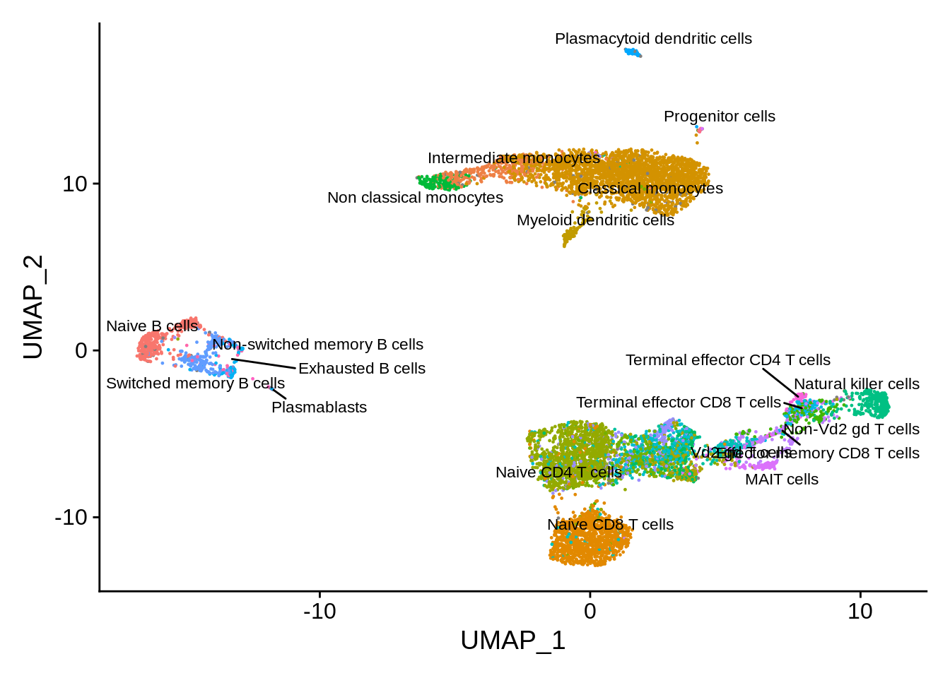
Comparing the labels obtained from the three sources, we can see many interesting discrepancies. Sorthing those out requires manual curation. However, many informative assignments can be seen. For example, small cluster 17 is repeatedly identified as plasma B cells. This distinct subpopulation displays markers such as CD38 and CD59.
FeaturePlot(srat,"CD38") + scale_colour_gradientn(colours = rev(brewer.pal(n = 11, name = "Spectral")))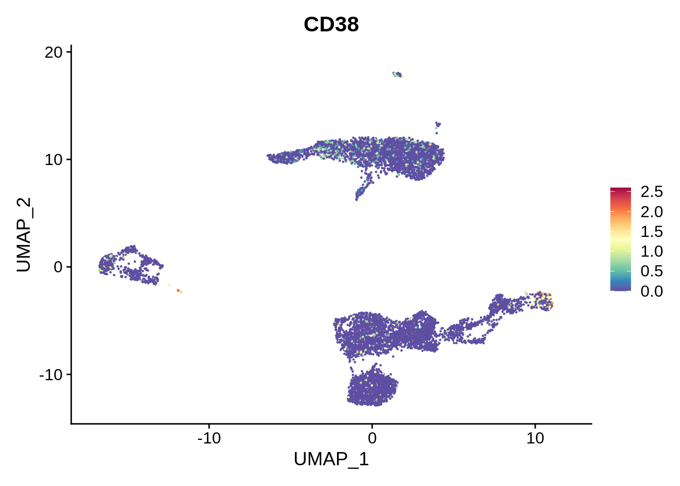
FeaturePlot(srat,"CD59") + scale_colour_gradientn(colours = rev(brewer.pal(n = 11, name = "Spectral")))
Similarly, cluster 13 is identified to be MAIT cells. Literature suggests that blood MAIT cells are characterized by high expression of CD161 (KLRB1), and chemokines like CXCR6. This indeed seems to be the case; however, this cell type is harder to evaluate.
FeaturePlot(srat,"KLRB1") + scale_colour_gradientn(colours = rev(brewer.pal(n = 11, name = "Spectral")))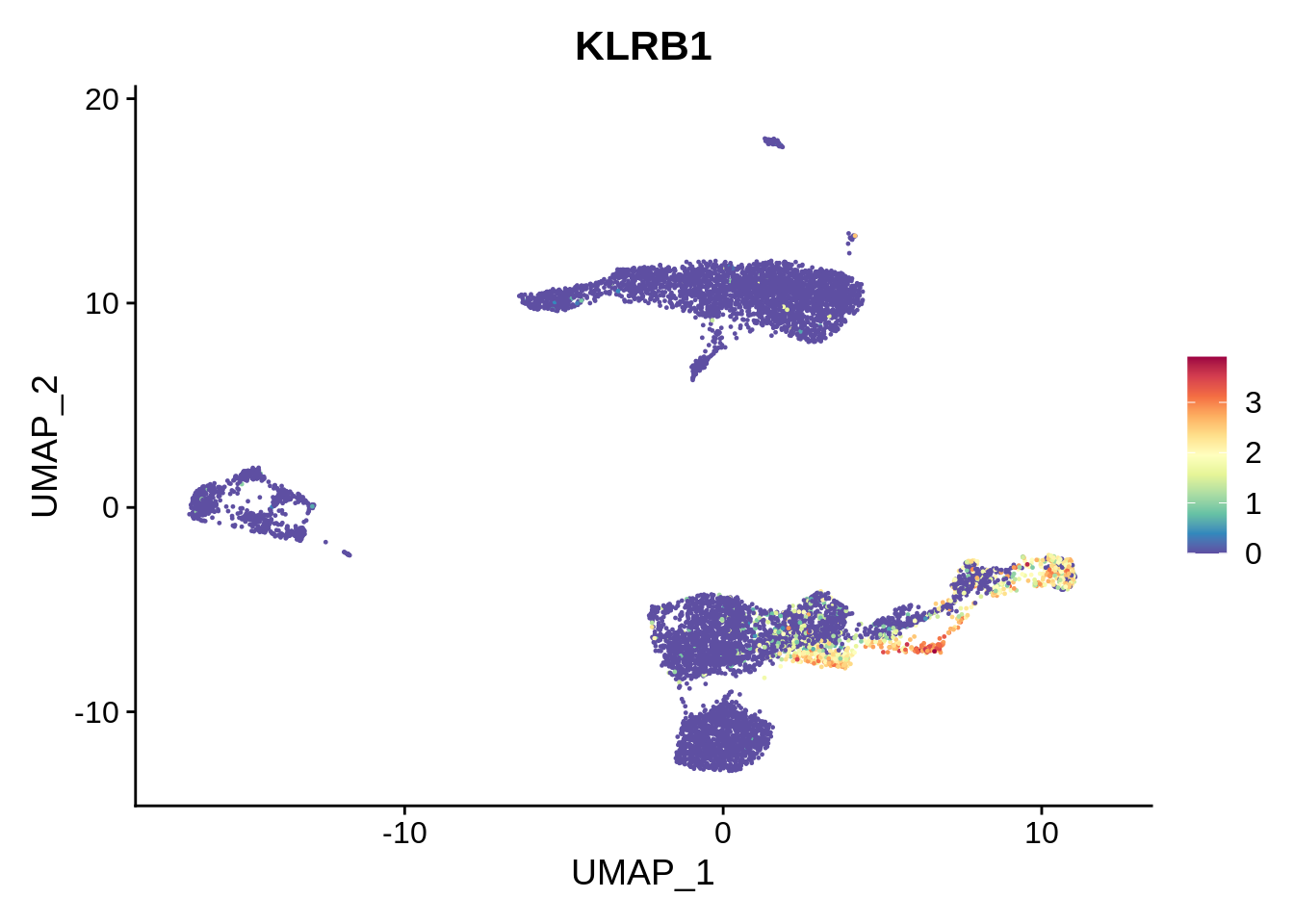
FeaturePlot(srat,"CXCR6") + scale_colour_gradientn(colours = rev(brewer.pal(n = 11, name = "Spectral")))
In general, even simple example of PBMC shows how complicated cell type assignment can be, and how much effort it requires. A detailed book on how to do cell type assignment / label transfer with singleR is available.
8.5.1 sessionInfo()
View session info
## R version 4.2.1 (2022-06-23)
## Platform: x86_64-pc-linux-gnu (64-bit)
## Running under: Ubuntu 20.04.2 LTS
##
## Matrix products: default
## BLAS:   /usr/lib/x86_64-linux-gnu/blas/libblas.so.3.9.0
## LAPACK: /usr/lib/x86_64-linux-gnu/lapack/liblapack.so.3.9.0
##
## locale:
##  [1] LC_CTYPE=en_US.UTF-8       LC_NUMERIC=C
##  [3] LC_TIME=en_US.UTF-8        LC_COLLATE=en_US.UTF-8
##  [5] LC_MONETARY=en_US.UTF-8    LC_MESSAGES=en_US.UTF-8
##  [7] LC_PAPER=en_US.UTF-8       LC_NAME=C
##  [9] LC_ADDRESS=C               LC_TELEPHONE=C
## [11] LC_MEASUREMENT=en_US.UTF-8 LC_IDENTIFICATION=C
##
## attached base packages:
## [1] stats4    stats     graphics  grDevices utils     datasets  methods
## [8] base
##
## other attached packages:
##  [1] SingleCellExperiment_1.18.0 RColorBrewer_1.1-3
##  [3] celldex_1.6.0               dplyr_1.0.9
##  [5] SingleR_1.10.0              SummarizedExperiment_1.26.1
##  [7] Biobase_2.56.0              GenomicRanges_1.48.0
##  [9] GenomeInfoDb_1.32.2         IRanges_2.30.0
## [11] S4Vectors_0.34.0            BiocGenerics_0.42.0
## [13] MatrixGenerics_1.8.1        matrixStats_0.62.0
## [15] ggplot2_3.3.6               sp_1.5-0
## [17] SeuratObject_4.1.0          Seurat_4.1.1
## [19] knitr_1.39
##
## loaded via a namespace (and not attached):
##   [1] utf8_1.2.2                    reticulate_1.25
##   [3] tidyselect_1.1.2              RSQLite_2.2.14
##   [5] AnnotationDbi_1.58.0          htmlwidgets_1.5.4
##   [7] grid_4.2.1                    BiocParallel_1.30.3
##   [9] Rtsne_0.16                    munsell_0.5.0
##  [11] ScaledMatrix_1.4.0            codetools_0.2-18
##  [13] ica_1.0-3                     future_1.26.1
##  [15] miniUI_0.1.1.1                withr_2.5.0
##  [17] spatstat.random_2.2-0         colorspace_2.0-3
##  [19] progressr_0.10.1              filelock_1.0.2
##  [21] highr_0.9                     ROCR_1.0-11
##  [23] tensor_1.5                    listenv_0.8.0
##  [25] labeling_0.4.2                GenomeInfoDbData_1.2.8
##  [27] polyclip_1.10-0               farver_2.1.1
##  [29] bit64_4.0.5                   rprojroot_2.0.3
##  [31] parallelly_1.32.0             vctrs_0.4.1
##  [33] generics_0.1.3                xfun_0.31
##  [35] BiocFileCache_2.4.0           R6_2.5.1
##  [37] ggbeeswarm_0.6.0              rsvd_1.0.5
##  [39] bitops_1.0-7                  spatstat.utils_2.3-1
##  [41] cachem_1.0.6                  DelayedArray_0.22.0
##  [43] assertthat_0.2.1              promises_1.2.0.1
##  [45] scales_1.2.0                  rgeos_0.5-9
##  [47] beeswarm_0.4.0                gtable_0.3.0
##  [49] beachmat_2.12.0               globals_0.15.1
##  [51] goftest_1.2-3                 rlang_1.0.4
##  [53] splines_4.2.1                 lazyeval_0.2.2
##  [55] spatstat.geom_2.4-0           BiocManager_1.30.18
##  [57] yaml_2.3.5                    reshape2_1.4.4
##  [59] abind_1.4-5                   httpuv_1.6.5
##  [61] tools_4.2.1                   bookdown_0.27
##  [63] ellipsis_0.3.2                spatstat.core_2.4-4
##  [65] jquerylib_0.1.4               ggridges_0.5.3
##  [67] Rcpp_1.0.9                    plyr_1.8.7
##  [69] sparseMatrixStats_1.8.0       zlibbioc_1.42.0
##  [71] purrr_0.3.4                   RCurl_1.98-1.7
##  [73] rpart_4.1.16                  deldir_1.0-6
##  [75] pbapply_1.5-0                 cowplot_1.1.1
##  [77] zoo_1.8-10                    ggrepel_0.9.1
##  [79] cluster_2.1.3                 here_1.0.1
##  [81] magrittr_2.0.3                glmGamPoi_1.8.0
##  [83] RSpectra_0.16-1               data.table_1.14.2
##  [85] scattermore_0.8               lmtest_0.9-40
##  [87] RANN_2.6.1                    fitdistrplus_1.1-8
##  [89] patchwork_1.1.1               mime_0.12
##  [91] evaluate_0.15                 xtable_1.8-4
##  [93] gridExtra_2.3                 compiler_4.2.1
##  [95] tibble_3.1.7                  KernSmooth_2.23-20
##  [97] crayon_1.5.1                  htmltools_0.5.2
##  [99] mgcv_1.8-40                   later_1.3.0
## [101] tidyr_1.2.0                   DBI_1.1.3
## [103] ExperimentHub_2.4.0           dbplyr_2.2.1
## [105] MASS_7.3-58                   rappdirs_0.3.3
## [107] Matrix_1.4-1                  cli_3.3.0
## [109] parallel_4.2.1                igraph_1.3.2
## [111] pkgconfig_2.0.3               plotly_4.10.0
## [113] spatstat.sparse_2.1-1         vipor_0.4.5
## [115] bslib_0.3.1                   XVector_0.36.0
## [117] stringr_1.4.0                 digest_0.6.29
## [119] sctransform_0.3.3             RcppAnnoy_0.0.19
## [121] spatstat.data_2.2-0           Biostrings_2.64.0
## [123] rmarkdown_2.14                leiden_0.4.2
## [125] uwot_0.1.11                   DelayedMatrixStats_1.18.0
## [127] curl_4.3.2                    shiny_1.7.1
## [129] lifecycle_1.0.1               nlme_3.1-157
## [131] jsonlite_1.8.0                BiocNeighbors_1.14.0
## [133] limma_3.52.2                  viridisLite_0.4.0
## [135] fansi_1.0.3                   pillar_1.7.0
## [137] lattice_0.20-45               ggrastr_1.0.1
## [139] KEGGREST_1.36.3               fastmap_1.1.0
## [141] httr_1.4.3                    survival_3.3-1
## [143] interactiveDisplayBase_1.34.0 glue_1.6.2
## [145] png_0.1-7                     BiocVersion_3.15.2
## [147] bit_4.0.4                     stringi_1.7.8
## [149] sass_0.4.1                    blob_1.2.3
## [151] BiocSingular_1.12.0           AnnotationHub_3.4.0
## [153] memoise_2.0.1                 irlba_2.3.5
## [155] future.apply_1.9.0