9 scRNA-seq Dataset Integration
9.1 Introduction
As more and more scRNA-seq datasets become available, carrying merged_seurat comparisons between them is key. There are two main approaches to comparing scRNASeq datasets. The first approach is “label-centric” which is focused on trying to identify equivalent cell-types/states across datasets by comparing individual cells or groups of cells. The other approach is “cross-dataset normalization” which attempts to computationally remove experiment-specific technical/biological effects so that data from multiple experiments can be combined and jointly analyzed.
The label-centric approach can be used with dataset with high-confidence cell-annotations, e.g. the Human Cell Atlas (HCA) (Regev et al. 2017) or the Tabula Muris (The Tabula Muris Consortium. 2018) once they are completed, to project cells or clusters from a new sample onto this reference to consider tissue composition and/or identify cells with novel/unknown identity. Conceptually, such projections are similar to the popular BLAST method (Altschul et al. 1990), which makes it possible to quickly find the closest match in a database for a newly identified nucleotide or amino acid sequence. The label-centric approach can also be used to compare datasets of similar biological origin collected by different labs to ensure that the annotation and the analysis is consistent.
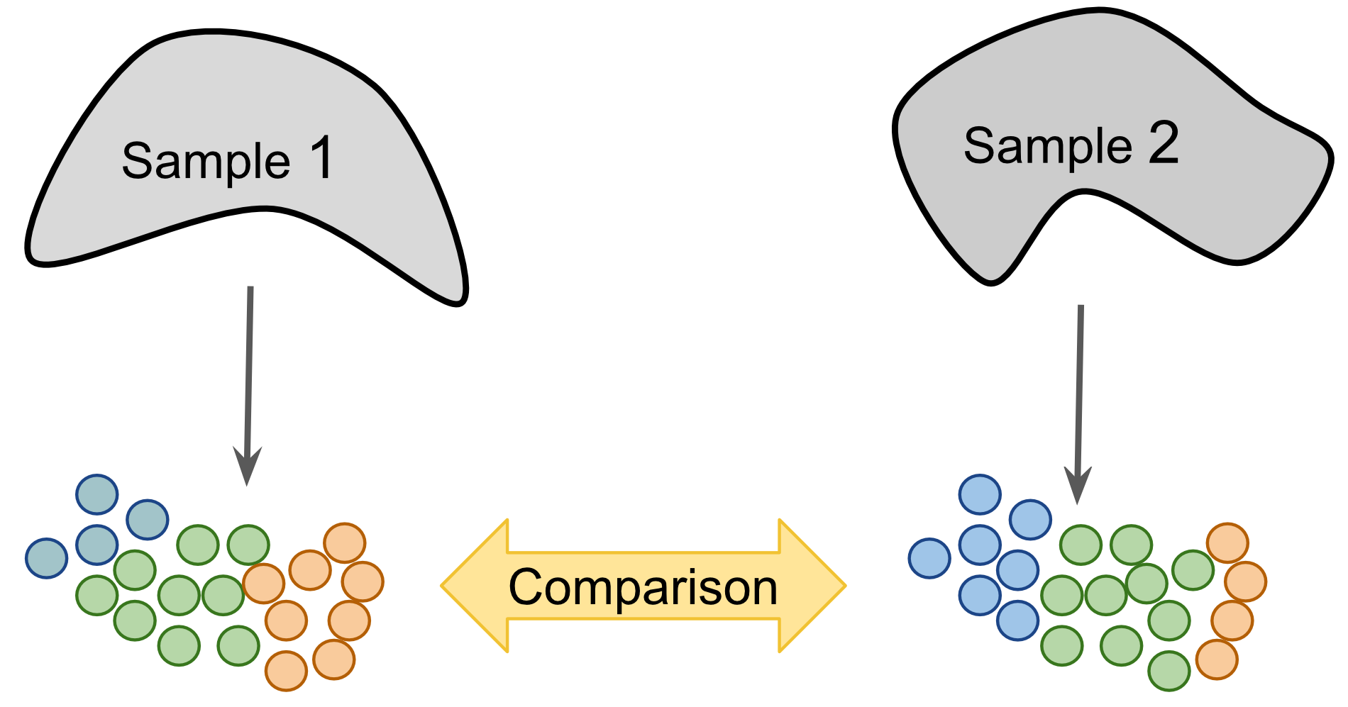
Figure 9.1: Label-centric dataset comparison can be used to compare the annotations of two different samples.
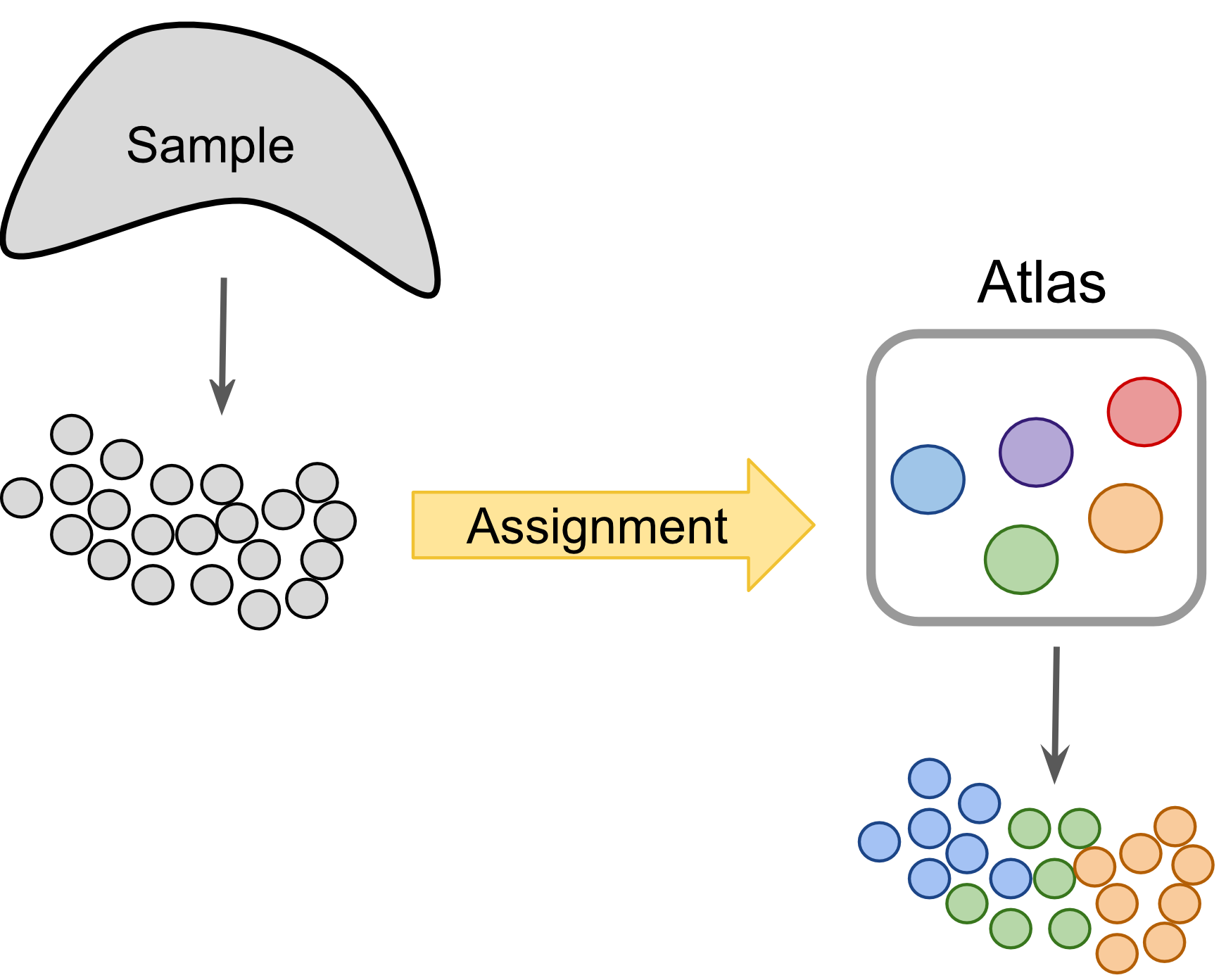
Figure 9.2: Label-centric dataset comparison can project cells from a new experiment onto an annotated reference.
The cross-dataset normalization approach can also be used to compare datasets of similar biological origin, unlike the label-centric approach it enables the join analysis of multiple datasets to facilitate the identification of rare cell-types which may to too sparsely sampled in each individual dataset to be reliably detected. However, cross-dataset normalization is not applicable to very large and diverse references since it assumes a significant portion of the biological variablility in each of the datasets overlaps with others.
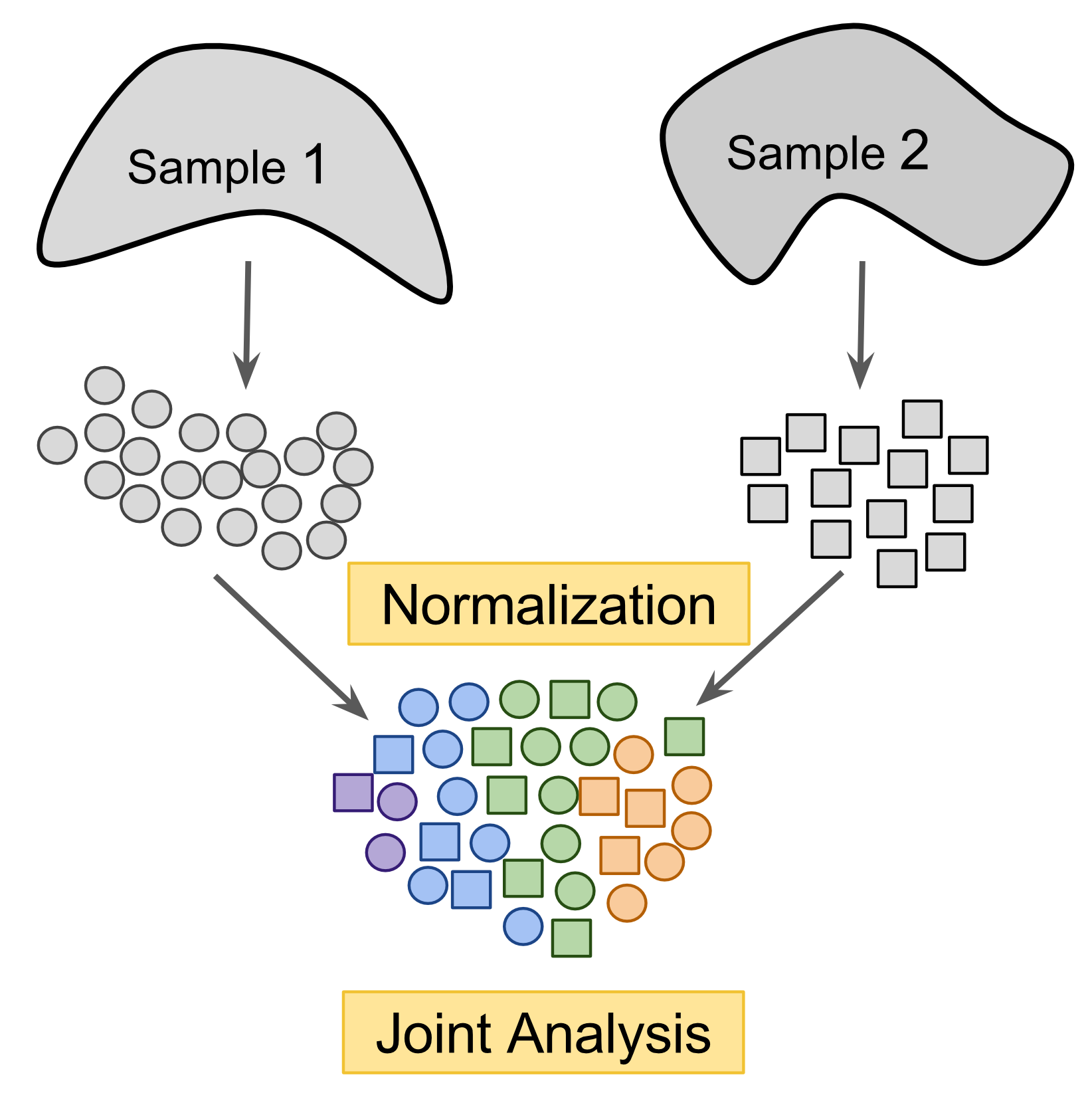
Figure 9.3: Cross-dataset normalization enables joint-analysis of 2+ scRNASeq datasets.
9.2 MNN-based methods
mnnCorrect corrects datasets to facilitate joint analysis. It order to account for differences in composition between two replicates or two different experiments it first matches invidual cells across experiments to find the overlaping biologicial structure. Using that overlap it learns which dimensions of expression correspond to the biological state and which dimensions correspond to batch/experiment effect; mnnCorrect assumes these dimensions are orthologal to each other in high dimensional expression space. Finally it removes the batch/experiment effects from the entire expression matrix to return the corrected matrix.
To match individual cells to each other across datasets, mnnCorrect uses the cosine distance to avoid library-size effect then identifies mututal nearest neighbours (k determines to neighbourhood size) across datasets. Only overlaping biological groups should have mutual nearest neighbours (see panel b below). However, this assumes that k is set to approximately the size of the smallest biological group in the datasets, but a k that is too low will identify too few mutual nearest-neighbour pairs to get a good estimate of the batch effect we want to remove.
Learning the biological/techncial effects is done with either singular value decomposition, similar to RUV we encounters in the batch-correction section, or with principal component analysis with the opitimized irlba package, which should be faster than SVD. The parameter svd.dim specifies how many dimensions should be kept to summarize the biological structure of the data, we will set it to three as we found three major groups using Metaneighbor above. These estimates may be futher adjusted by smoothing (sigma) and/or variance adjustment (var.adj).
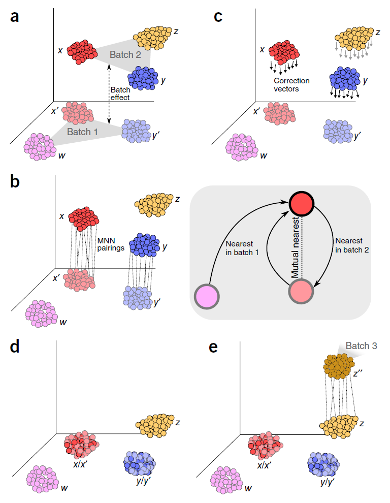
Figure 9.4: Scheme of a mutual nearest neighbor (MNN) integration approach
9.3 Cannonical Correlation Analysis (Seurat v3)
The Seurat package contains another correction method for combining multiple datasets, called CCA. However, unlike mnnCorrect it doesn’t correct the expression matrix itself directly. Instead Seurat finds a lower dimensional subspace for each dataset then corrects these subspaces. Also different from mnnCorrect, Seurat only combines a single pair of datasets at a time.
Seurat uses gene-gene correlations to identify the biological structure in the dataset with a method called canonical correlation analysis (CCA). Seurat learns the shared structure to the gene-gene correlations and then evaluates how well each cell fits this structure. Cells which must better described by a data-specific dimensionality reduction method than by the shared correlation structure are assumed to represent dataset-specific cell-types/states and are discarded before aligning the two datasets. Finally the two datasets are aligned using ‘warping’ algorithms which normalize the low-dimensional representations of each dataset in a way that is robust to differences in population density.
9.4 Practical Integration of Real Datasets
There are several benchmarks published recently (Chazarra-Gil et al, 2021; Tran et al, 2020; Luecken et al, 2020). One of the most detailed publications (Tran 2020) compared 14 methods of scRNA-seq dataset integration using multiple simulated and real datasets of various size and complexity.
According to the benchmark, Harmony, LIGER (that more recently became rliger), and Seurat (v3) have performed best. We will illustrate the performance of these three methods in two tasks: 1) integrating closely related 3’ and 5’ PBMC datasets; 2) integrating only partially overlapping datasets, namely whole blood (including erythrocytes and neutrophils), and 3’ PBMC dataset.
Let’s load all the necessary libraries:
library(Seurat)
library(SeuratDisk)
library(SeuratWrappers)

library(patchwork)
library(harmony)
library(rliger)
library(reshape2)
library(RColorBrewer)
library(dplyr)
Also, let’s source a custom function we’ve written to visualize the distribution of cells of different datasets per cluster, alongside cluster sizes:
source("utils/custom_seurat_functions.R")9.5 Seurat v3, 3’ vs 5’ 10k PBMC
Let’s load the filtered Cell Ranger h5 matrices downloaded from 10x Genomics data repository. These can also be downloaded using the commands below.
download.file("https://cf.10xgenomics.com/samples/cell-exp/4.0.0/Parent_NGSC3_DI_PBMC/Parent_NGSC3_DI_PBMC_filtered_feature_bc_matrix.h5",
              destfile = "3p_pbmc10k_filt.h5")
download.file("https://cf.10xgenomics.com/samples/cell-vdj/5.0.0/sc5p_v2_hs_PBMC_10k/sc5p_v2_hs_PBMC_10k_filtered_feature_bc_matrix.h5",
              destfile = "5p_pbmc10k_filt.h5")
Let’s read the data and create the appropriate Seurat objects. Note that 5’ dataset has other assays - namely, VDJ data.
matrix_3p <- Read10X_h5("data/update/3p_pbmc10k_filt.h5",use.names = T)
matrix_5p <- Read10X_h5("data/update/5p_pbmc10k_filt.h5",use.names = T)$`Gene Expression`

srat_3p   <- CreateSeuratObject(matrix_3p,project = "pbmc10k_3p")
srat_5p   <- CreateSeuratObject(matrix_5p,project = "pbmc10k_5p")
Now let’s remove matrices to save memory:
rm(matrix_3p)
rm(matrix_5p)
Let’s calculate the fractions of mitochondrial genes and ribosomal proteins, and do quick-and-dirty filtering of the datasets:
srat_3p[["percent.mt"]]  <- PercentageFeatureSet(srat_3p, pattern = "^MT-")
srat_3p[["percent.rbp"]] <- PercentageFeatureSet(srat_3p, pattern = "^RP[SL]")
srat_5p[["percent.mt"]]  <- PercentageFeatureSet(srat_5p, pattern = "^MT-")
srat_5p[["percent.rbp"]] <- PercentageFeatureSet(srat_5p, pattern = "^RP[SL]")

VlnPlot(srat_3p, features = c("nFeature_RNA","nCount_RNA","percent.mt","percent.rbp"), ncol = 4)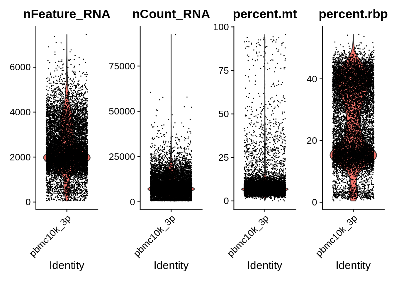
VlnPlot(srat_5p, features = c("nFeature_RNA","nCount_RNA","percent.mt","percent.rbp"), ncol = 4)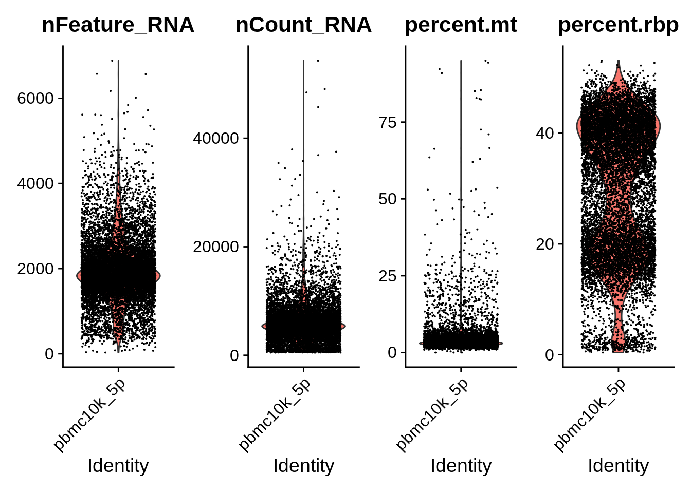
Now, let’s look how similar the annotations are, i.e. compare gene names. Turns out they are identical: both used the latest Cell Ranger annotation, GRCh38-2020A.
table(rownames(srat_3p) %in% rownames(srat_5p)) ##
## TRUE
## 36601Quick filtering of the datasets removes dying cells and putative doublets:
srat_3p <- subset(srat_3p, subset = nFeature_RNA > 500 & nFeature_RNA < 5000 & percent.mt < 15)
srat_5p <- subset(srat_5p, subset = nFeature_RNA > 500 & nFeature_RNA < 5000 & percent.mt < 10)
Now, let’s follow Seurat vignette for integration. To do this we need to make a simple R list of the two objects, and normalize/find HVG for each:
pbmc_list <- list()
pbmc_list[["pbmc10k_3p"]] <- srat_3p
pbmc_list[["pbmc10k_5p"]] <- srat_5p

for (i in 1:length(pbmc_list)) {
  pbmc_list[[i]] <- NormalizeData(pbmc_list[[i]], verbose = F)
  pbmc_list[[i]] <- FindVariableFeatures(pbmc_list[[i]], selection.method = "vst", nfeatures = 2000, verbose = F)
}
After this, we use the two following Seurat commands to find integration anchors and actually perform integration. This takes about 10 min:
pbmc_anchors <- FindIntegrationAnchors(object.list = pbmc_list, dims = 1:30)## Warning in CheckDuplicateCellNames(object.list = object.list): Some cell names
## are duplicated across objects provided. Renaming to enforce unique cell names.## Computing 2000 integration features## Scaling features for provided objects## Finding all pairwise anchors## Running CCA## Merging objects## Finding neighborhoods## Finding anchors## Found 21626 anchors## Filtering anchors## Retained 8832 anchorspbmc_seurat <- IntegrateData(anchorset = pbmc_anchors, dims = 1:30)## Merging dataset 1 into 2## Extracting anchors for merged samples## Finding integration vectors## Finding integration vector weights## Integrating dataLet’s remove all the datastructures we’re not using to save the RAM:
rm(pbmc_list)
rm(pbmc_anchors)
Seurat integration creates a unified object that contains both original data (‘RNA’ assay) as well as integrated data (‘integrated’ assay). Let’s set the assay to RNA and visualize the datasets before integration.
DefaultAssay(pbmc_seurat) <- "RNA"Let’s do normalization, HVG finding, scaling, PCA, and UMAP on the un-integrated (RNA) assay:
pbmc_seurat <- NormalizeData(pbmc_seurat, verbose = F)
pbmc_seurat <- FindVariableFeatures(pbmc_seurat, selection.method = "vst", nfeatures = 2000, verbose = F)
pbmc_seurat <- ScaleData(pbmc_seurat, verbose = F)
pbmc_seurat <- RunPCA(pbmc_seurat, npcs = 30, verbose = F)
pbmc_seurat <- RunUMAP(pbmc_seurat, reduction = "pca", dims = 1:30, verbose = F)
## Warning: The default method for RunUMAP has changed from calling Python UMAP via reticulate to the R-native UWOT using the cosine metric
## To use Python UMAP via reticulate, set umap.method to 'umap-learn' and metric to 'correlation'
## This message will be shown once per sessionUMAP plot of the datasets before integration shows clear separation. Note that we can use patchwork syntax with Seurat plotting functions:
DimPlot(pbmc_seurat,reduction = "umap") + plot_annotation(title = "10k 3' PBMC and 10k 5' PBMC cells, before integration")
Now let’s change the assay to integrated and do the same do the same thing in the integrated assay (it’s already normalized and HVGs are selected):
DefaultAssay(pbmc_seurat) <- "integrated"
pbmc_seurat <- ScaleData(pbmc_seurat, verbose = F)
pbmc_seurat <- RunPCA(pbmc_seurat, npcs = 30, verbose = F)
pbmc_seurat <- RunUMAP(pbmc_seurat, reduction = "pca", dims = 1:30, verbose = F)
Finally, let’s plot the integrated UMAP:
DimPlot(pbmc_seurat, reduction = "umap") + plot_annotation(title = "10k 3' PBMC and 10k 5' PBMC cells, after integration (Seurat 3)")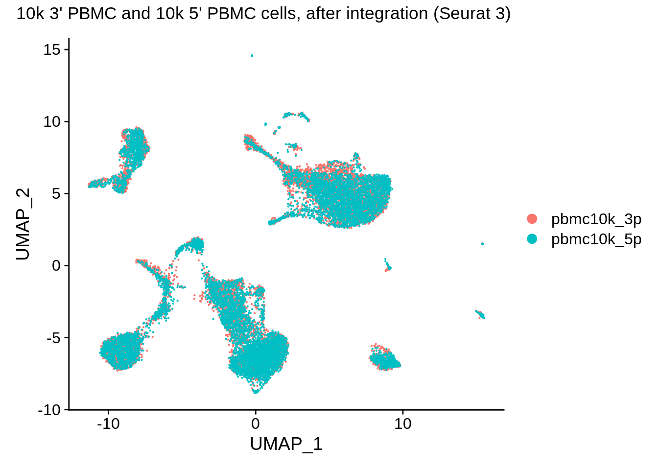
The data are visibly very nicely integrated. Let’s try a split plot, which should make the comparison easier:
DimPlot(pbmc_seurat, reduction = "umap", split.by = "orig.ident") + NoLegend()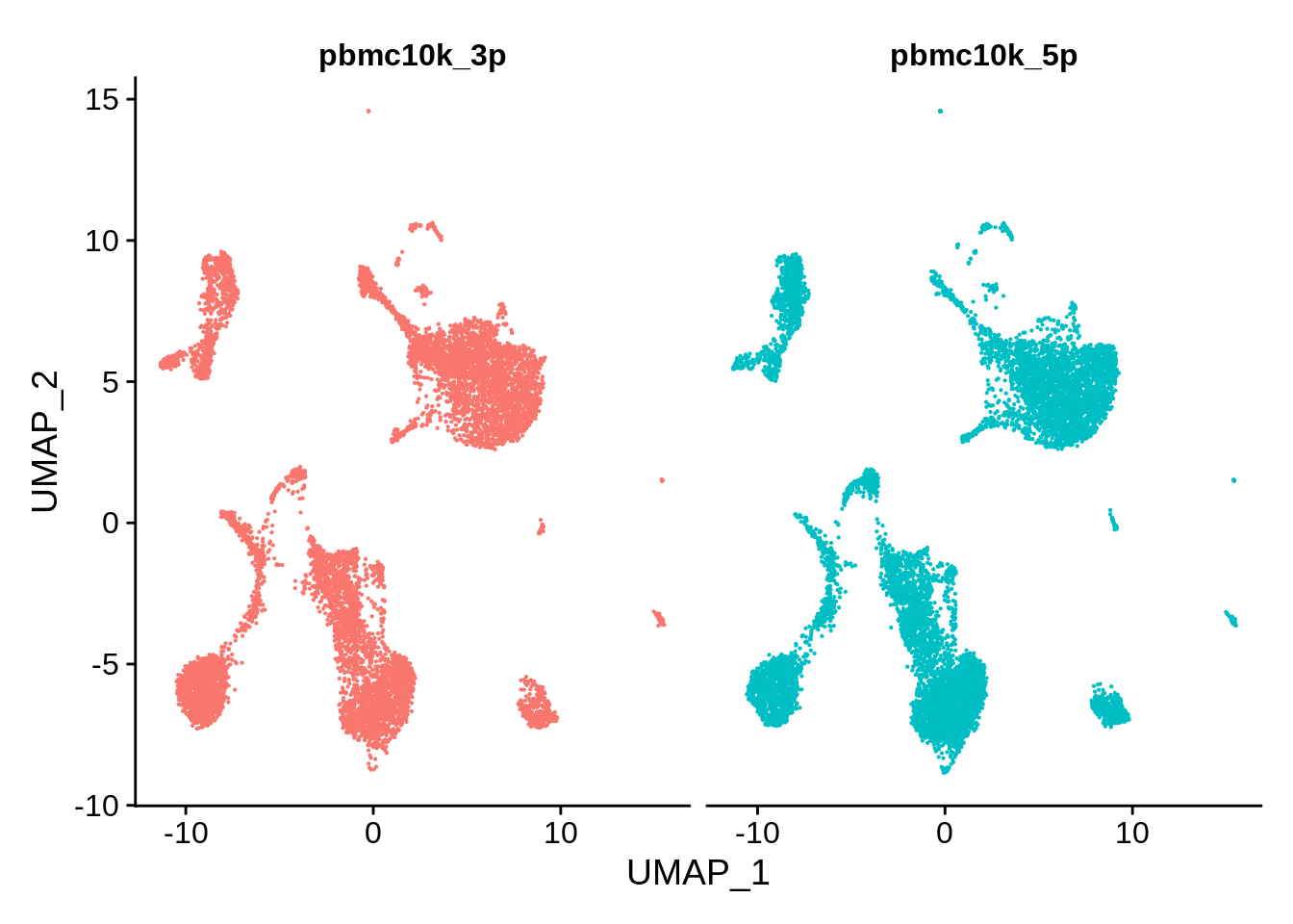
Now let’s cluster the integrated matrix and look how clusters are distributed between the two sets:
pbmc_seurat <- FindNeighbors(pbmc_seurat, dims = 1:30, k.param = 10, verbose = F)
pbmc_seurat <- FindClusters(pbmc_seurat, verbose = F)
DimPlot(pbmc_seurat,label = T) + NoLegend()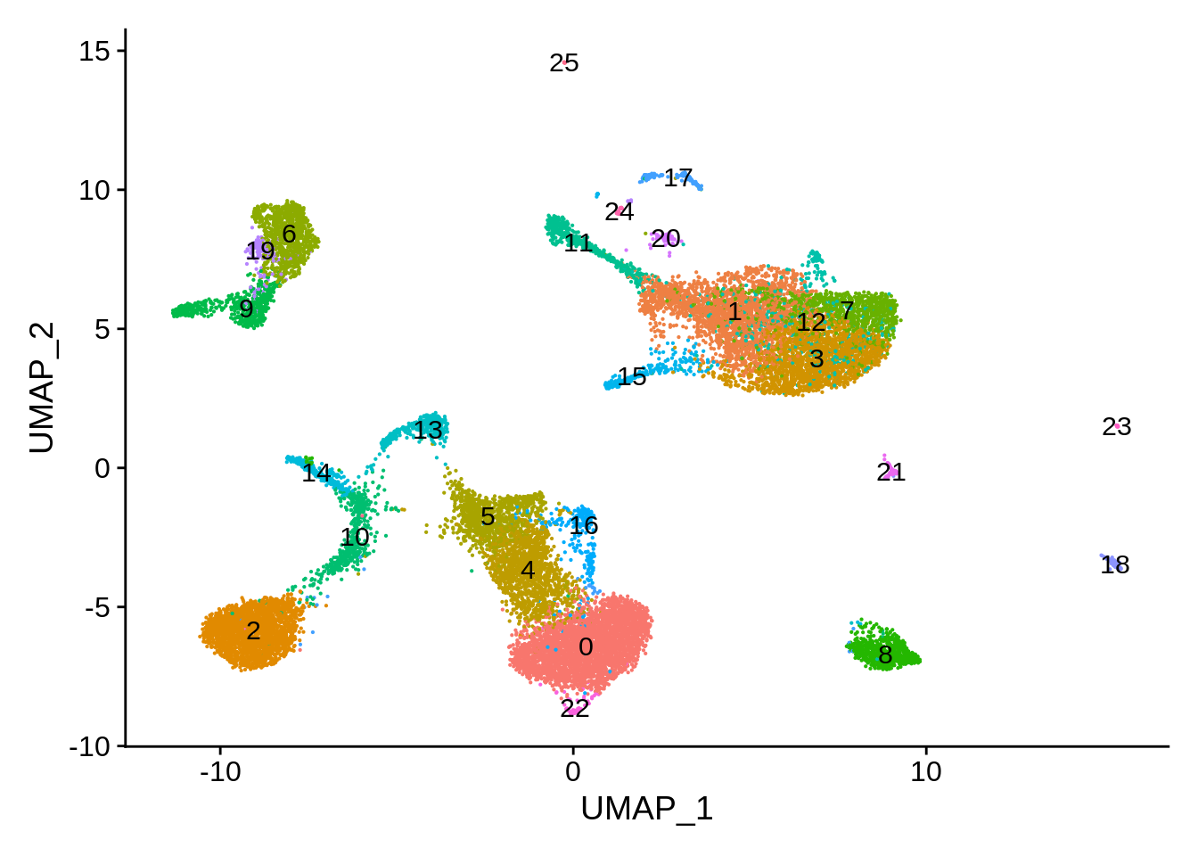
We can now calculate the number of cells in each cluster that came for either 3’ or the 5’ dataset:
count_table <- table(pbmc_seurat@meta.data$seurat_clusters, pbmc_seurat@meta.data$orig.ident)
count_table
##
## pbmc10k_3p pbmc10k_5p
## 0 1313 2140
## 1 1427 945
## 2 1214 994
## 3 898 1110
## 4 612 769
## 5 576 437
## 6 401 603
## 7 338 646
## 8 311 403
## 9 359 223
## 10 251 292
## 11 347 131
## 12 202 240
## 13 136 288
## 14 251 61
## 15 109 190
## 16 118 143
## 17 76 92
## 18 93 61
## 19 55 87
## 20 35 35
## 21 24 43
## 22 13 40
## 23 15 10
## 24 14 5
## 25 2 12Let’s plot the distribution among clusters using our custom function:
plot_integrated_clusters(pbmc_seurat) ## Using cluster as id variables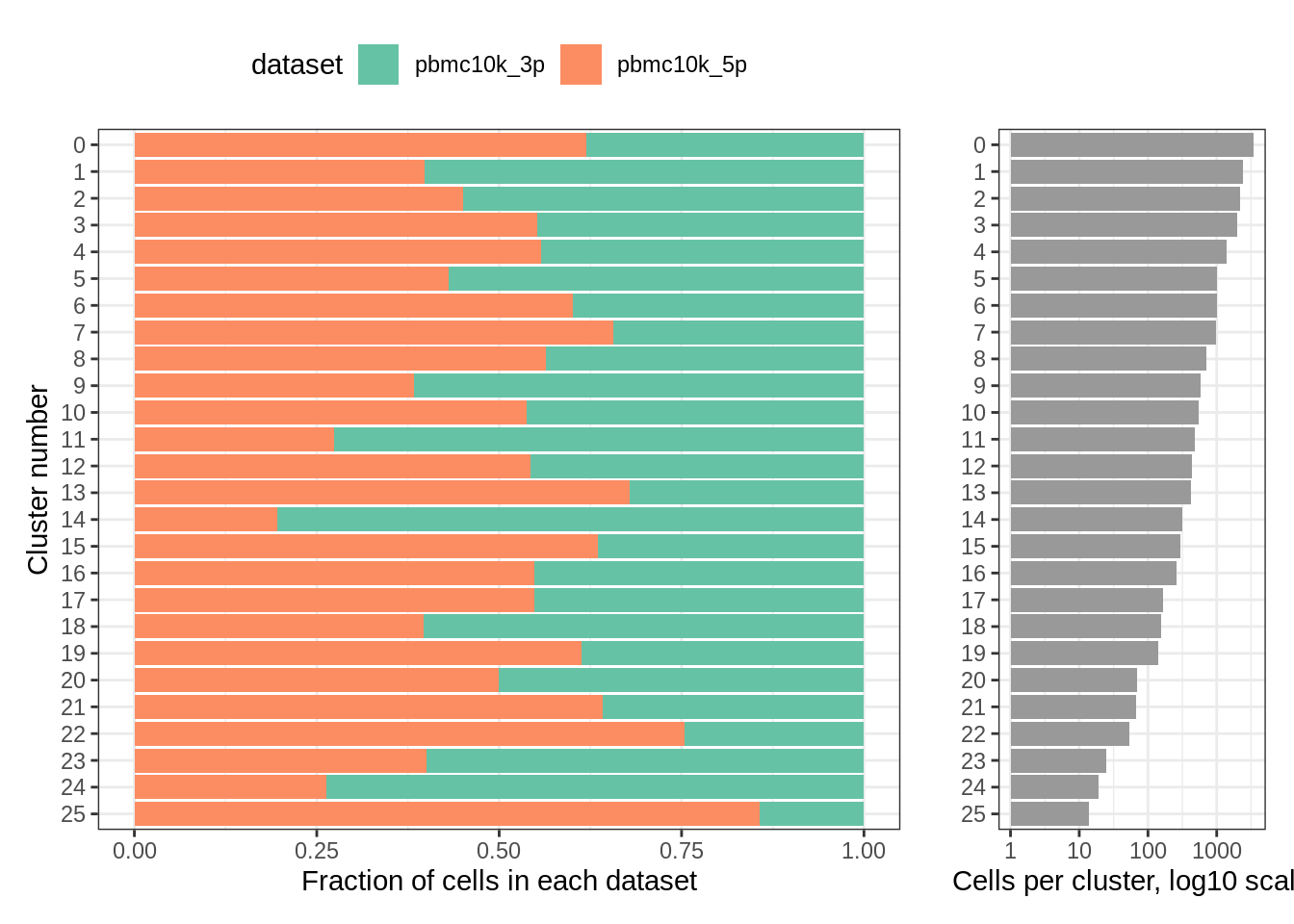
rm(pbmc_seurat)9.6 Harmony, 3’ vs 5’ 10k PBMC
Using harmony is much faster than pretty much any other method, and was found to perform quite well in a recent benchmark. There also are convenient wrappers for interfacing with Seurat. Let’s first merge the objects (without integration). Note the message about the matching cell barcodes:
pbmc_harmony <- merge(srat_3p,srat_5p)## Warning in CheckDuplicateCellNames(object.list = objects): Some cell names are
## duplicated across objects provided. Renaming to enforce unique cell names.Now let’s do the same as we did before:
pbmc_harmony <- NormalizeData(pbmc_harmony, verbose = F)
pbmc_harmony <- FindVariableFeatures(pbmc_harmony, selection.method = "vst", nfeatures = 2000, verbose = F)
pbmc_harmony <- ScaleData(pbmc_harmony, verbose = F)
pbmc_harmony <- RunPCA(pbmc_harmony, npcs = 30, verbose = F)
pbmc_harmony <- RunUMAP(pbmc_harmony, reduction = "pca", dims = 1:30, verbose = F)
Let’s plot the “before” plot again:
DimPlot(pbmc_harmony,reduction = "umap") + plot_annotation(title = "10k 3' PBMC and 10k 5' PBMC cells, before integration")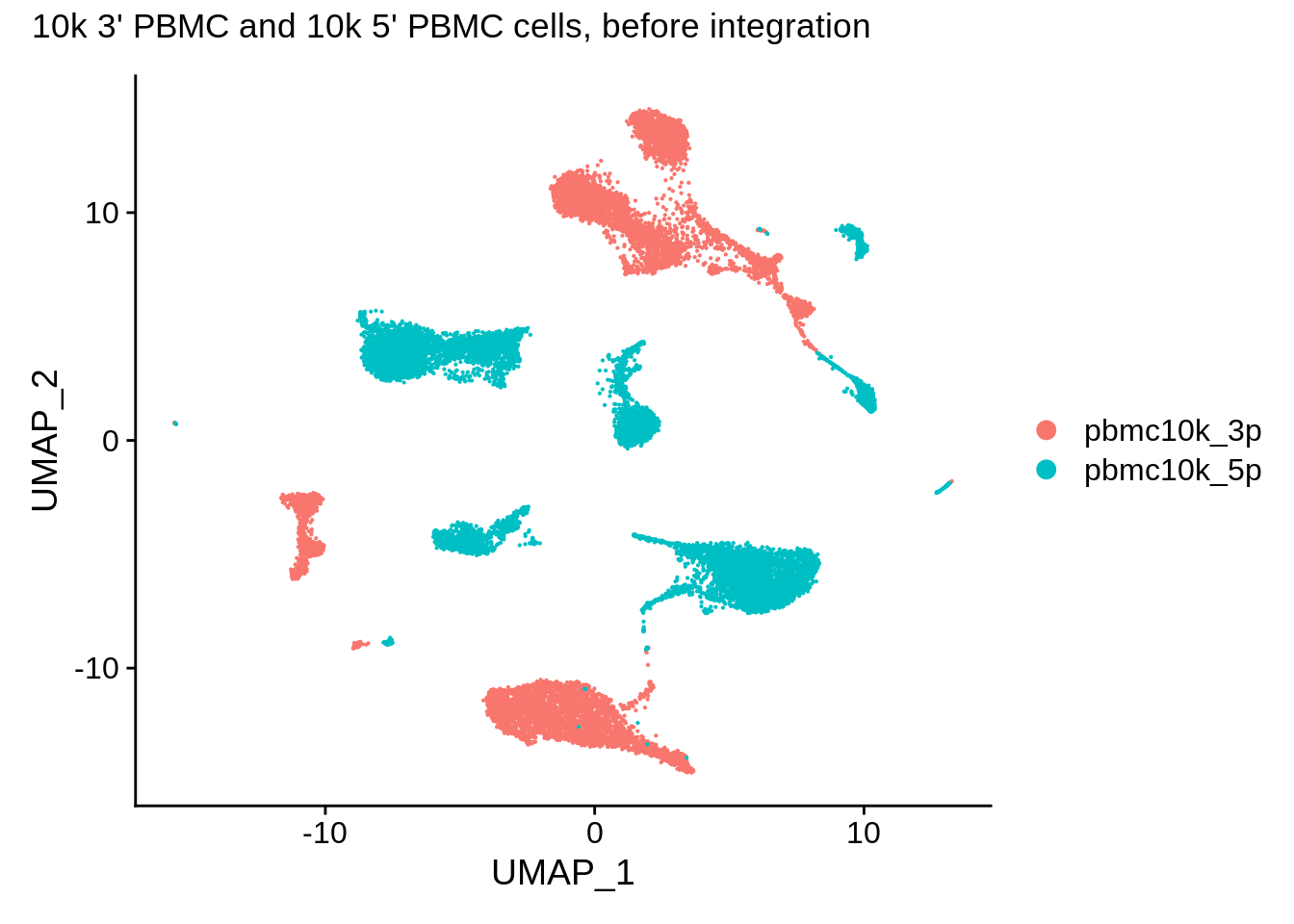
Use RunHarmony to run it on the combined Seurat object using orig.ident as batch:
pbmc_harmony <- pbmc_harmony %>% RunHarmony("orig.ident", plot_convergence = T)## Harmony 1/10## Harmony 2/10## Harmony 3/10## Harmony 4/10## Harmony 5/10## Harmony converged after 5 iterations## Warning: Invalid name supplied, making object name syntactically valid. New
## object name is Seurat..ProjectDim.RNA.harmony; see ?make.names for more details
## on syntax validity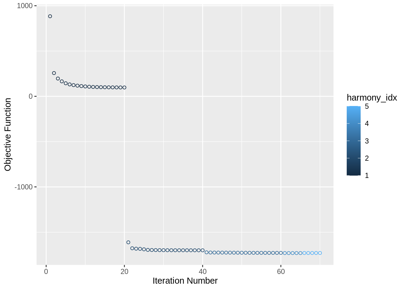
Check the generated embeddings:
harmony_embeddings <- Embeddings(pbmc_harmony, 'harmony')
harmony_embeddings[1:5, 1:5]
## harmony_1 harmony_2 harmony_3 harmony_4 harmony_5
## AAACCCACATAACTCG-1_1 -9.206607 -2.351619 -2.374652 -1.897186 -1.011885
## AAACCCACATGTAACC-1_1 7.124223 21.600131 -0.292039 1.530283 -5.792142
## AAACCCAGTGAGTCAG-1_1 -18.134725 3.405369 5.256459 4.220001 3.961466
## AAACGAACAGTCAGTT-1_1 -18.103262 15.279955 12.301681 -18.115094 31.785955
## AAACGAACATTCGGGC-1_1 11.097966 -2.330278 -2.723953 1.546468 1.552332Check the PCA plot after:
p1 <- DimPlot(object = pbmc_harmony, reduction = "harmony", pt.size = .1, group.by = "orig.ident") + NoLegend()
p2 <- VlnPlot(object = pbmc_harmony, features = "harmony_1", group.by = "orig.ident", pt.size = .1) + NoLegend()
plot_grid(p1,p2)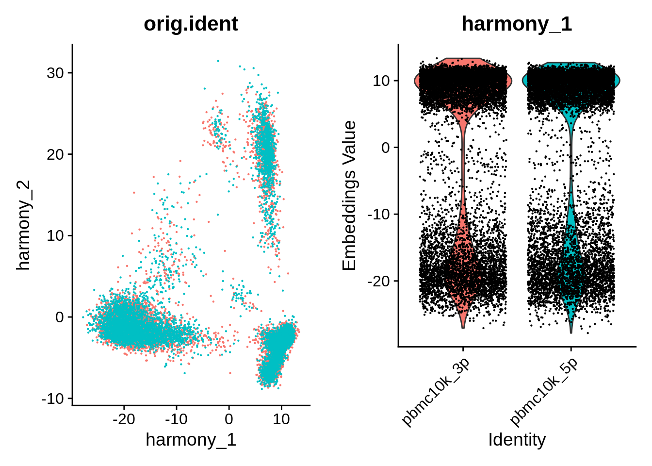
Do UMAP and clustering:
pbmc_harmony <- pbmc_harmony %>%
  RunUMAP(reduction = "harmony", dims = 1:30, verbose = F) %>%
  FindNeighbors(reduction = "harmony", k.param = 10, dims = 1:30) %>%
  FindClusters() %>%
  identity()
## Computing nearest neighbor graph## Computing SNN## Modularity Optimizer version 1.3.0 by Ludo Waltman and Nees Jan van Eck
##
## Number of nodes: 19190
## Number of edges: 280811
##
## Running Louvain algorithm...
## Maximum modularity in 10 random starts: 0.8952
## Number of communities: 26
## Elapsed time: 3 secondsFinally, so same UMAP plots of integrated datasets as above:
pbmc_harmony <- SetIdent(pbmc_harmony,value = "orig.ident")
DimPlot(pbmc_harmony,reduction = "umap") + plot_annotation(title = "10k 3' PBMC and 10k 5' PBMC cells, after integration (Harmony)")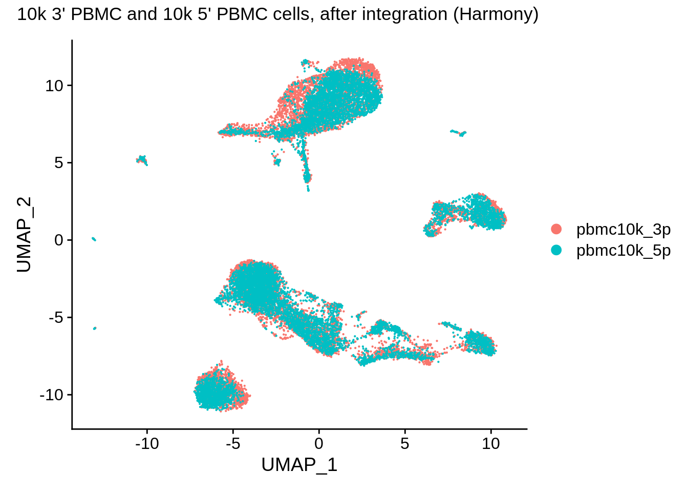
DimPlot(pbmc_harmony, reduction = "umap", group.by = "orig.ident", pt.size = .1, split.by = 'orig.ident') + NoLegend()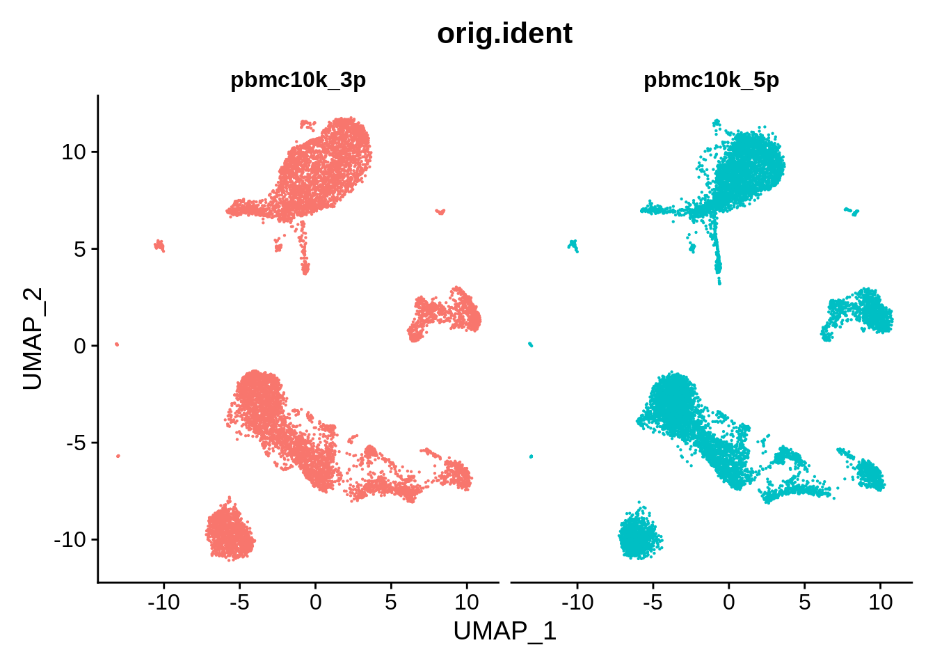
These look a bit worse than ones from Seurat:
pbmc_harmony <- SetIdent(pbmc_harmony,value = "seurat_clusters")
DimPlot(pbmc_harmony,label = T) + NoLegend()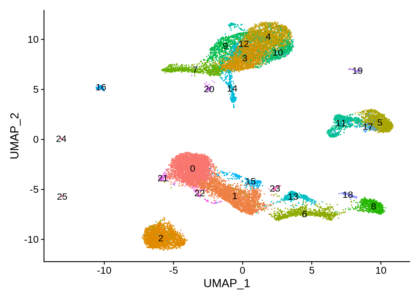
Finally, let’s take a look at the cluster content:
plot_integrated_clusters(pbmc_harmony)## Using cluster as id variables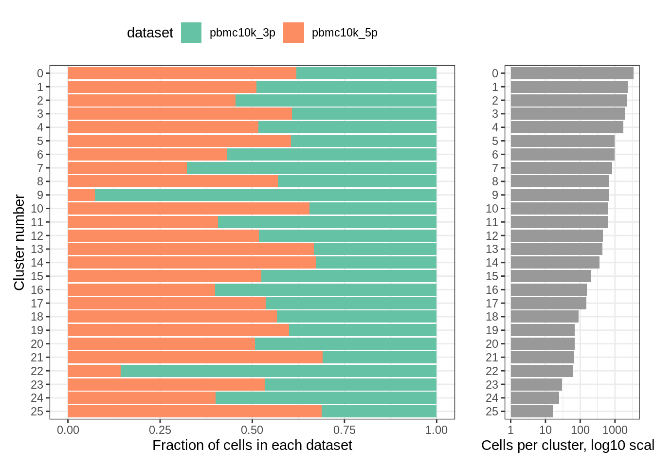
rm(pbmc_harmony)Clusters and their content look pretty similar to what we obtained after Seurat integration. For a more detailed analysis, we would need cell type assignments.
9.7 LIGER, 3’ vs 5’ 10k PBMC
Similarly to other methods, we make a unified object and normalize/HVG/scale it. LIGER does not center data when scaling, hence the do.center option in ScaleData). The last two functions are wrappers that run rliger using orig.ident as a batch variable.
pbmc_liger <- merge(srat_3p,srat_5p)## Warning in CheckDuplicateCellNames(object.list = objects): Some cell names are
## duplicated across objects provided. Renaming to enforce unique cell names.pbmc_liger <- NormalizeData(pbmc_liger)
pbmc_liger <- FindVariableFeatures(pbmc_liger)
pbmc_liger <- ScaleData(pbmc_liger, split.by = "orig.ident", do.center = F)## Scaling data matrix## Scaling data from split pbmc10k_3p## Scaling data from split pbmc10k_5ppbmc_liger <- RunOptimizeALS(pbmc_liger, k = 30, lambda = 5, split.by = "orig.ident") ## this one takes a while##
|
| | 0%
|
|== | 3%
|
|===== | 7%
|
|======= | 10%
|
|========= | 13%
|
|============ | 17%
|
|============== | 20%
|
|================ | 23%
|
|=================== | 27%
|
|===================== | 30%
|
|======================= | 33%
|
|========================== | 37%
|
|============================ | 40%
|
|============================== | 43%
|
|================================= | 47%
|
|=================================== | 50%
|
|===================================== | 53%
|
|======================================== | 57%
|
|========================================== | 60%
|
|============================================ | 63%
|
|=============================================== | 67%
|
|================================================= | 70%
|
|=================================================== | 73%
|
|====================================================== | 77%
|
|======================================================== | 80%
|
|========================================================== | 83%
|
|============================================================= | 87%
|
|=============================================================== | 90%
|
|================================================================= | 93%
|
|==================================================================== | 97%
|
|======================================================================| 100%
## Finished in 9.525399 mins, 30 iterations.
## Max iterations set: 30.
## Final objective delta: 1.924923e-05.
## Best results with seed 1.## Warning: No columnames present in cell embeddings, setting to 'riNMF_1:30'pbmc_liger <- RunQuantileNorm(pbmc_liger, split.by = "orig.ident")You can optionally perform Louvain clustering (FindNeighbors and FindClusters) after RunQuantileNorm - we’ll do this as well to compare the results to the previous integration approaches. We use the same parameters (k = 10 for neighbors, default resolution for Louvain clustering).
pbmc_liger <- FindNeighbors(pbmc_liger,reduction = "iNMF",k.param = 10,dims = 1:30)## Computing nearest neighbor graph## Computing SNNpbmc_liger <- FindClusters(pbmc_liger)## Modularity Optimizer version 1.3.0 by Ludo Waltman and Nees Jan van Eck
##
## Number of nodes: 19190
## Number of edges: 281100
##
## Running Louvain algorithm...
## Maximum modularity in 10 random starts: 0.8986
## Number of communities: 29
## Elapsed time: 1 secondsAs previously, let’s do dimensionality reduction and plotting:
pbmc_liger    <- RunUMAP(pbmc_liger, dims = 1:ncol(pbmc_liger[["iNMF"]]), reduction = "iNMF", verbose = F)
pbmc_liger    <- SetIdent(pbmc_liger,value = "orig.ident")
DimPlot(pbmc_liger,reduction = "umap") + plot_annotation(title = "10k 3' PBMC and 10k 5' PBMC cells, after integration (LIGER)")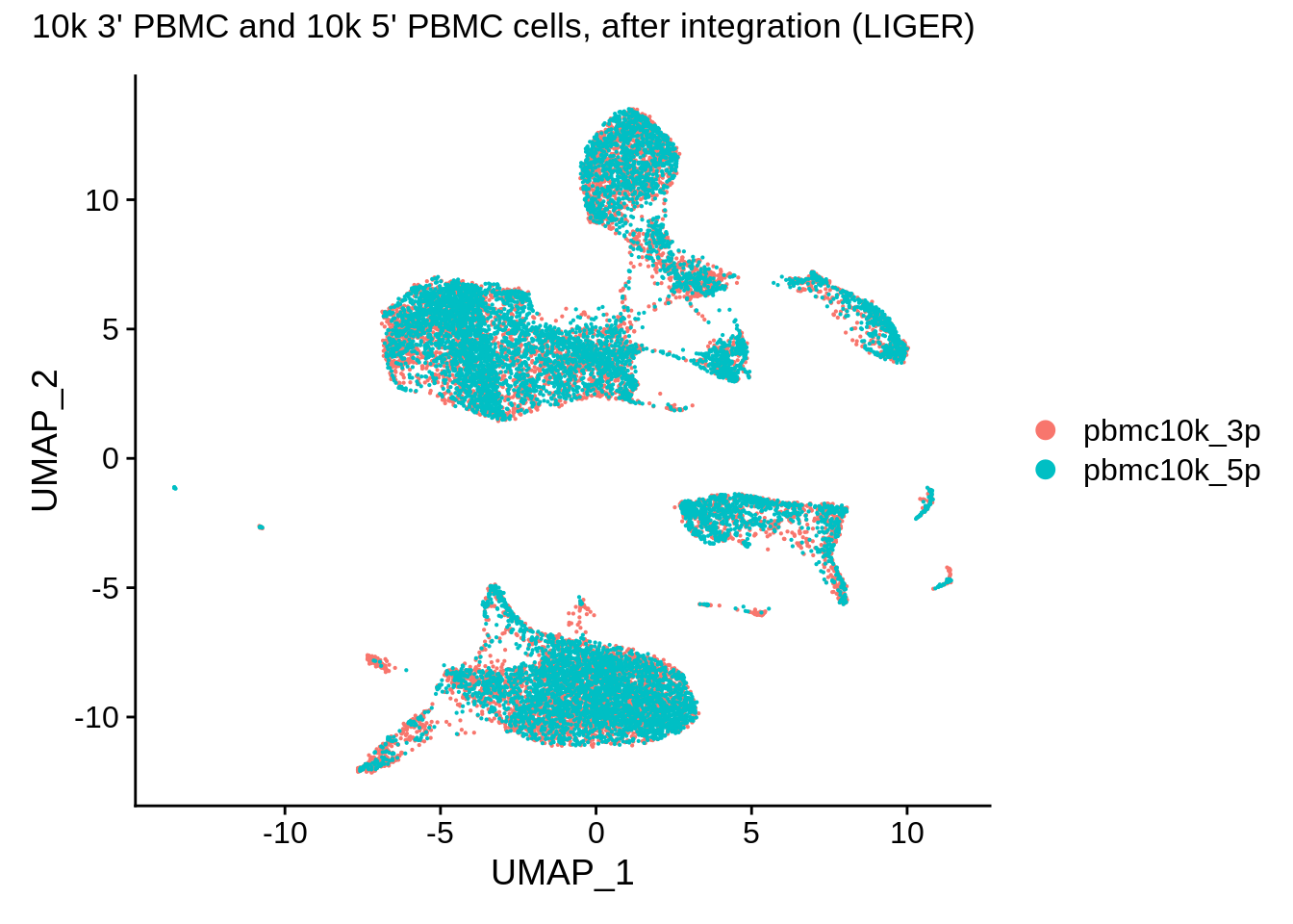
DimPlot(pbmc_liger, reduction = "umap", group.by = "orig.ident", pt.size = .1, split.by = 'orig.ident') + NoLegend()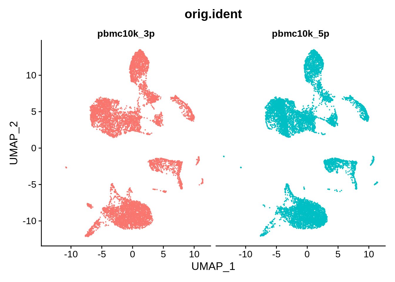
Clustering appears to be somewhat finer with the LIGER-integrated data:
pbmc_liger <- SetIdent(pbmc_liger,value = "seurat_clusters")
DimPlot(pbmc_liger,reduction = "umap",label = T) + NoLegend()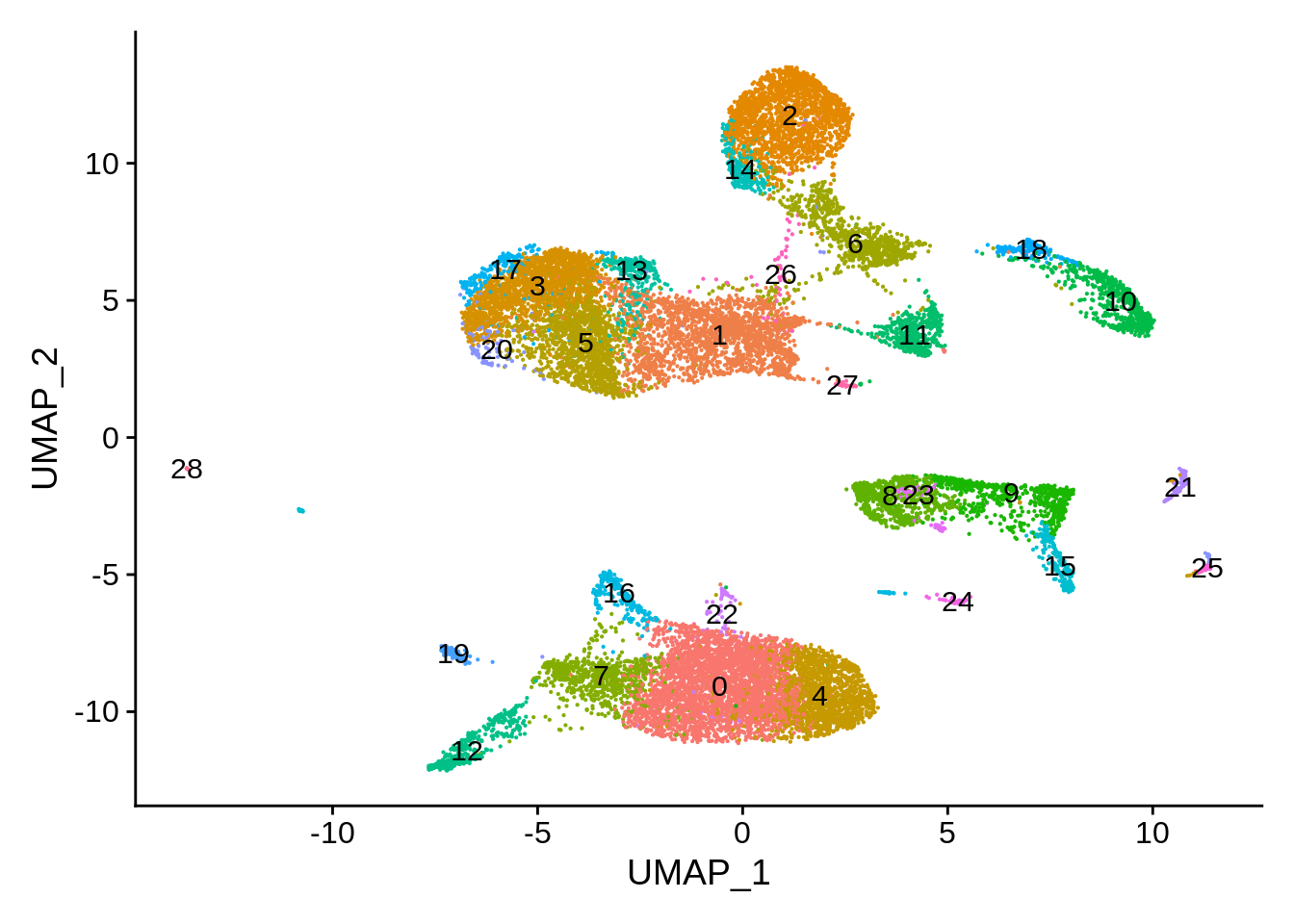
The clusters look pretty different, and per-cluster distribution seems to confirm this (two clusters were deemed unique to 3’ and 5’ dataset, respectively):
plot_integrated_clusters(pbmc_liger)## Using cluster as id variables
rm(pbmc_liger)
rm(srat_3p)
rm(srat_5p)
9.8 Seurat v3, 3’ 10k PBMC cells and whole blood STRT-Seq
Although we already have all the necessary files in our /data folder, we can download the necessary files from GEO database:
download.file("https://ftp.ncbi.nlm.nih.gov/geo/series/GSE149nnn/GSE149938/suppl/GSE149938_umi_matrix.csv.gz",
              destfile = "GSE149938_umi_matrix.csv.gz")
download.file("https://cf.10xgenomics.com/samples/cell-exp/4.0.0/Parent_NGSC3_DI_PBMC/Parent_NGSC3_DI_PBMC_filtered_feature_bc_matrix.h5",
              destfile = "3p_pbmc10k_filt.h5")
umi_gz <- gzfile("data/update/GSE149938_umi_matrix.csv.gz",'rt')
umi <- read.csv(umi_gz,check.names = F,quote = "")
matrix_3p <- Read10X_h5("data/update/3p_pbmc10k_filt.h5",use.names = T)Next, let’s make Seurat objects and re-define some of the metadata columns (GEO dataset simply puts the cell type into the orig.ident slot, which will interfere with what we want to do next):
srat_wb <- CreateSeuratObject(t(umi),project = "whole_blood")## Warning: Non-unique features (rownames) present in the input matrix, making
## uniquesrat_3p <- CreateSeuratObject(matrix_3p,project = "pbmc10k_3p")
rm(umi_gz)
rm(umi)
rm(matrix_3p)colnames(srat_wb@meta.data)[1] <- "cell_type"
srat_wb@meta.data$orig.ident <- "whole_blood"
srat_wb@meta.data$orig.ident <- as.factor(srat_wb@meta.data$orig.ident)
head(srat_wb[[]])## cell_type nCount_RNA nFeature_RNA orig.ident
## BNK_spBM1_L1_bar25 BNK 24494 1869 whole_blood
## BNK_spBM1_L1_bar26 BNK 61980 2051 whole_blood
## BNK_spBM1_L1_bar27 BNK 124382 3872 whole_blood
## BNK_spBM1_L1_bar28 BNK 8144 1475 whole_blood
## BNK_spBM1_L1_bar29 BNK 53612 2086 whole_blood
## BNK_spBM1_L1_bar30 BNK 33582 2038 whole_bloodDo basic quality control. STRT-Seq is quite different from 10x and has a lot more detected genes per cell. Also, for some reason we don’t have the MT genes in the quantified matrix of the whole blood dataset. That’s unfortunate, but not critical.
srat_wb <- SetIdent(srat_wb,value = "orig.ident")

srat_wb[["percent.mt"]] <- PercentageFeatureSet(srat_wb, pattern = "^MT-")
srat_wb[["percent.rbp"]] <- PercentageFeatureSet(srat_wb, pattern = "^RP[SL]")
srat_3p[["percent.mt"]] <- PercentageFeatureSet(srat_3p, pattern = "^MT-")
srat_3p[["percent.rbp"]] <- PercentageFeatureSet(srat_3p, pattern = "^RP[SL]")

VlnPlot(srat_wb, features = c("nFeature_RNA","nCount_RNA","percent.mt","percent.rbp"), ncol = 4)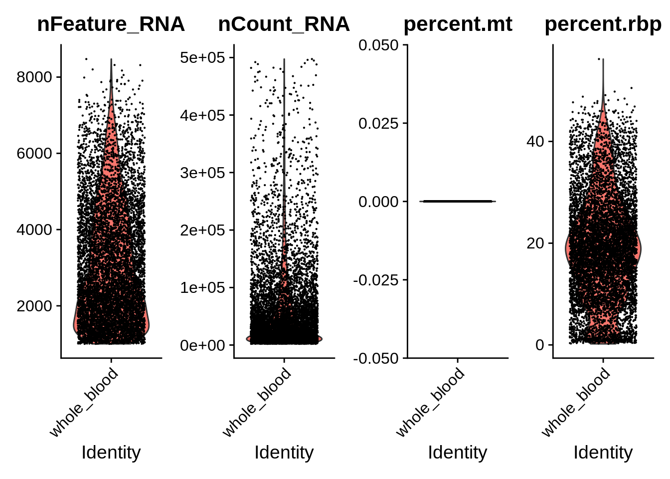
VlnPlot(srat_3p, features = c("nFeature_RNA","nCount_RNA","percent.mt","percent.rbp"), ncol = 4)
The annotation that was used to process the GEO whole blood dataset is quite different from the Cell Ranger GRCh38-2020A. Let’s see how many common genes are there:
table(rownames(srat_3p) %in% rownames(srat_wb))##
## FALSE TRUE
## 18050 18551common_genes <- rownames(srat_3p)[rownames(srat_3p) %in% rownames(srat_wb)]Let’s filter the cells with too high or too low number of genes, or too high MT gene content. Also, let’s limit the individual matrices to common genes only:
srat_3p <- subset(srat_3p, subset = nFeature_RNA > 500 & nFeature_RNA < 5000 & percent.mt < 15)
srat_wb <- subset(srat_wb, subset = nFeature_RNA > 1000 & nFeature_RNA < 6000)

srat_3p <- srat_3p[rownames(srat_3p) %in% common_genes,]
srat_wb <- srat_wb[rownames(srat_wb) %in% common_genes,]
As previously for Seurat v3, let’s make a list and normalize/find HVG for each object:
wb_list <- list()
wb_list[["pbmc10k_3p"]]   <- srat_3p
wb_list[["whole_blood"]]  <- srat_wb

for (i in 1:length(wb_list)) {
  wb_list[[i]] <- NormalizeData(wb_list[[i]], verbose = F)
  wb_list[[i]] <- FindVariableFeatures(wb_list[[i]], selection.method = "vst", nfeatures = 2000, verbose = F)
}
Here we actually do the integration. Seurat 3 does it in two steps.
wb_anchors <- FindIntegrationAnchors(object.list = wb_list, dims = 1:30)## Computing 2000 integration features## Scaling features for provided objects## Finding all pairwise anchors## Running CCA## Merging objects## Finding neighborhoods## Finding anchors## Found 11353 anchors## Filtering anchors## Retained 3276 anchorswb_seurat <- IntegrateData(anchorset = wb_anchors, dims = 1:30)## Merging dataset 2 into 1## Extracting anchors for merged samples## Finding integration vectors## Finding integration vector weights## Integrating datarm(wb_list)
rm(wb_anchors)Let’s do the basic processing and visualization of the uncorrected dataset:
DefaultAssay(wb_seurat) <- "RNA"
wb_seurat <- NormalizeData(wb_seurat, verbose = F)
wb_seurat <- FindVariableFeatures(wb_seurat, selection.method = "vst", nfeatures = 2000, verbose = F)
wb_seurat <- ScaleData(wb_seurat, verbose = F)
wb_seurat <- RunPCA(wb_seurat, npcs = 30, verbose = F)
wb_seurat <- RunUMAP(wb_seurat, reduction = "pca", dims = 1:30, verbose = F)

DimPlot(wb_seurat,reduction = "umap") + plot_annotation(title = "10k 3' PBMC and whole blood, before integration")
Now, let’s take a look at the integrated dataset (it’s already normalized and HVGs are selected):
DefaultAssay(wb_seurat) <- "integrated"
wb_seurat <- ScaleData(wb_seurat, verbose = F)
wb_seurat <- RunPCA(wb_seurat, npcs = 30, verbose = F)
wb_seurat <- RunUMAP(wb_seurat, reduction = "pca", dims = 1:30, verbose = F)

DimPlot(wb_seurat, reduction = "umap") + plot_annotation(title = "10k 3' PBMC and white blood cells, after integration (Seurat 3)")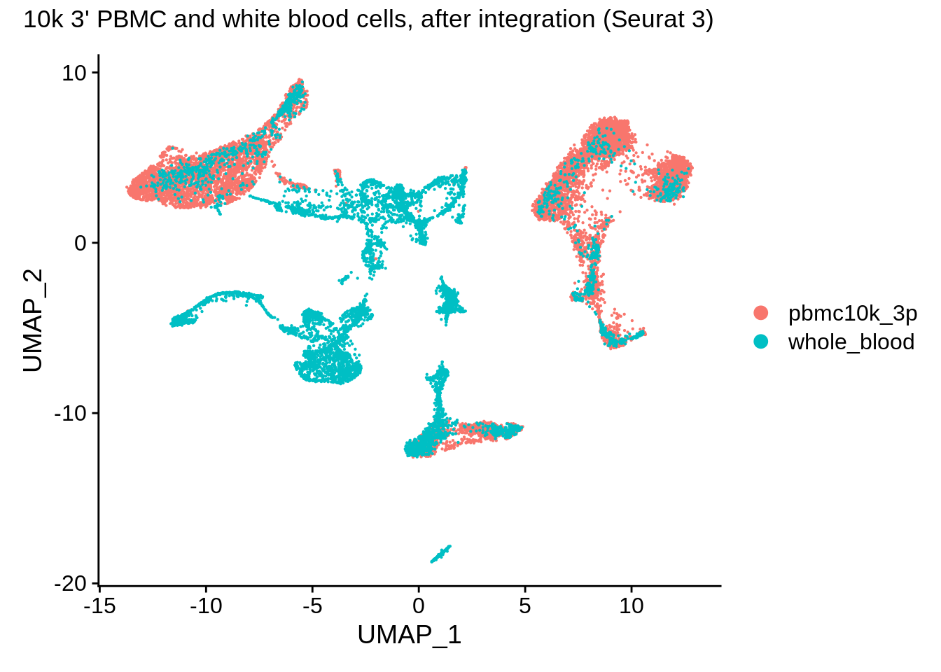
Let’s look at some markers:
FeaturePlot(wb_seurat,c("MS4A1","LYZ","NKG7","PPBP","LTF","HBA1","FCER1A","IL7R","FCGR3B")) & scale_colour_gradientn(colours = rev(brewer.pal(n = 11, name = "Spectral")))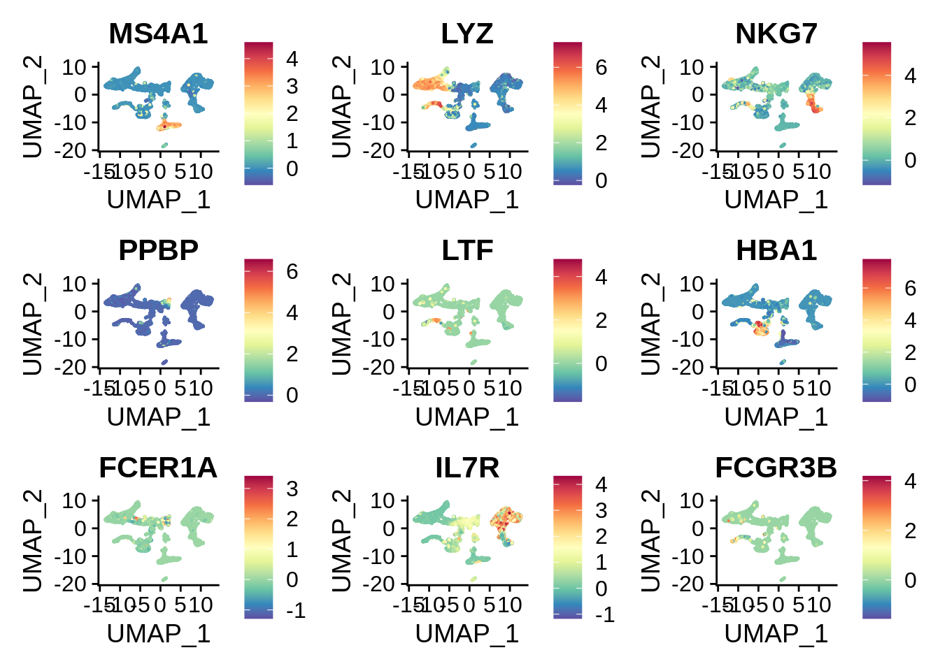
From the plot we can see that there are some significant cell types that are absent from PBMC dataset, but exist in the whole blood dataset. LTF gene is the most prominent marker of neutrophils, and HBA1 is a hemoglobin gene expressed in erythrocytes.
Now let’s cluster the integrated matrix and look how clusters are distributed between the two sets:
wb_seurat <- FindNeighbors(wb_seurat, dims = 1:30, k.param = 10, verbose = F)
wb_seurat <- FindClusters(wb_seurat, verbose = F)
DimPlot(wb_seurat,label = T) + NoLegend()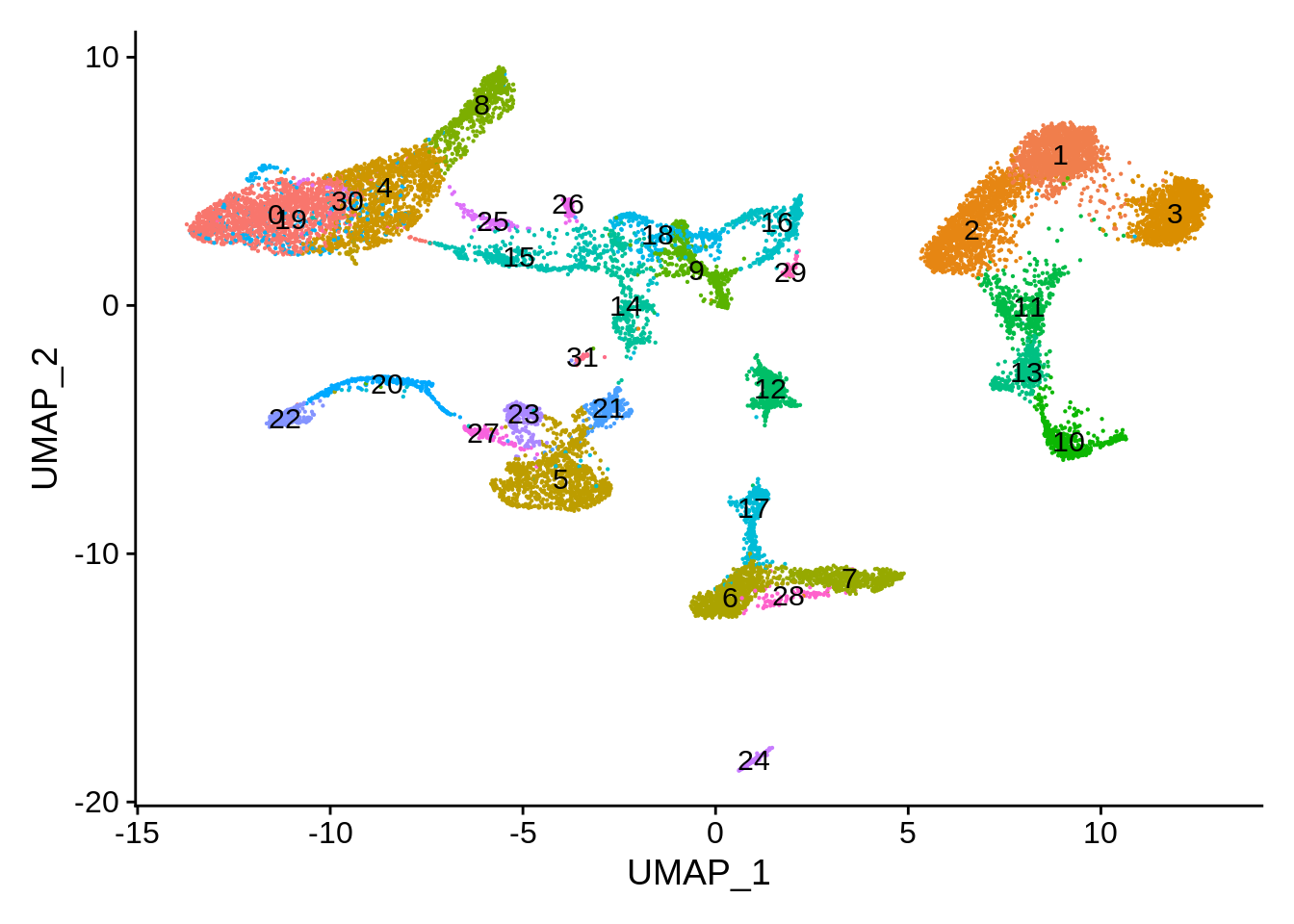
Cluster composition shows many clusters unique to the whole blood dataset:
count_table <- table(wb_seurat@meta.data$seurat_clusters, wb_seurat@meta.data$orig.ident)
count_table
##
## pbmc10k_3p whole_blood
## 0 1426 237
## 1 1385 71
## 2 1264 130
## 3 1211 112
## 4 1115 145
## 5 0 1052
## 6 355 467
## 7 377 211
## 8 386 199
## 9 0 550
## 10 343 157
## 11 390 82
## 12 0 441
## 13 283 125
## 14 7 388
## 15 3 380
## 16 19 362
## 17 4 367
## 18 2 316
## 19 297 13
## 20 0 308
## 21 0 265
## 22 0 222
## 23 0 221
## 24 15 179
## 25 106 22
## 26 93 19
## 27 0 103
## 28 77 3
## 29 0 50
## 30 32 2
## 31 0 32plot_integrated_clusters(wb_seurat)## Using cluster as id variables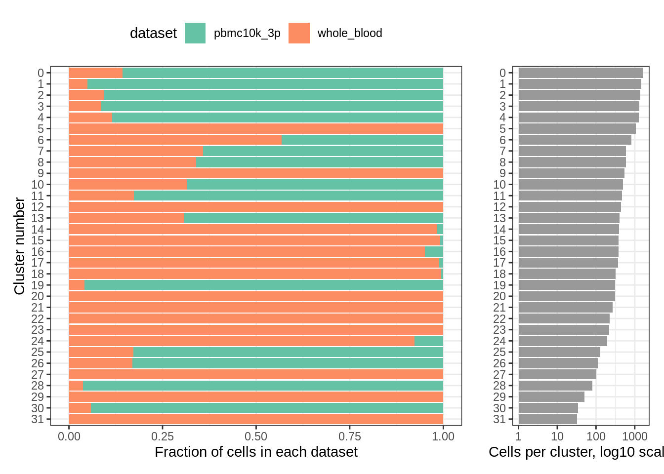
We can take advantage of the metadata that was present in GSE149938:
meta <- wb_seurat[[]]
table(meta[meta$seurat_clusters == '5',]$cell_type) ## erythrocytes
##
## BNK CMP ery immB MEP MLP preB proB toxiNK
## 1 2 1040 3 1 1 2 1 1table(meta[meta$seurat_clusters == '20',]$cell_type) ## neutrophils##
## BNK CLP CMP HSC immB kineNK matureN metaN MLP myeN
## 2 2 1 1 1 55 1 7 1 99
## plasma proN toxiNK
## 1 136 1table(meta[meta$seurat_clusters == '24',]$cell_type) ## plasma##
## ery naiB plasma
## 11 2 166table(meta[meta$seurat_clusters == '16',]$cell_type) ## platelets##
## BNK CLP CMP ery HSC LMPP matureN MEP MPP NKP
## 1 3 61 4 72 1 1 144 74 1rm(wb_seurat)9.9 Harmony, 3’ 10k PBMC cells and whole blood STRT-Seq
Similarly to the previous approaches, let’s make a merged Seurat dataset, normalize and process it:
wb_harmony    <- merge(srat_3p,srat_wb)

wb_harmony <- NormalizeData(wb_harmony, verbose = F)
wb_harmony <- FindVariableFeatures(wb_harmony, selection.method = "vst", nfeatures = 2000, verbose = F)
wb_harmony <- ScaleData(wb_harmony, verbose = F)
wb_harmony <- RunPCA(wb_harmony, npcs = 30, verbose = F)
wb_harmony <- RunUMAP(wb_harmony, reduction = "pca", dims = 1:30, verbose = F)
We can take a look at the PCA plot for a change, as well as distributions along the first principal component:
p1 <- DimPlot(object = wb_harmony, reduction = "pca", pt.size = .1, group.by = "orig.ident") + NoLegend()
p2 <- VlnPlot(object = wb_harmony, features = "PC_1", group.by = "orig.ident", pt.size = .1) + NoLegend()
plot_grid(p1,p2)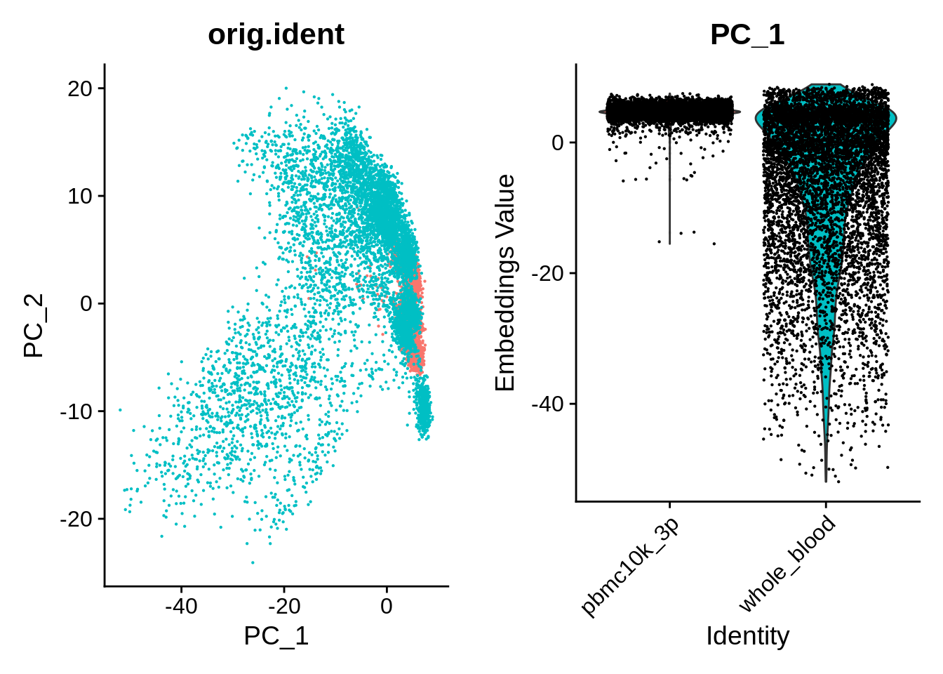
UMAP also shows clear differences between the datasets:
DimPlot(wb_harmony,reduction = "umap") + plot_annotation(title = "10k 3' PBMC and whole blood, before integration")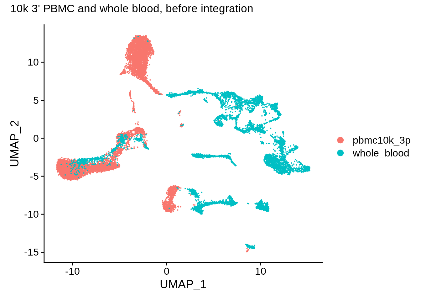
Let’s run harmony using a simple wrapper named RunHarmony from SeuratWrappers library:
wb_harmony <- wb_harmony %>% RunHarmony("orig.ident", plot_convergence = T)## Harmony 1/10## Harmony 2/10## Harmony 3/10## Harmony converged after 3 iterations## Warning: Invalid name supplied, making object name syntactically valid. New
## object name is Seurat..ProjectDim.RNA.harmony; see ?make.names for more details
## on syntax validity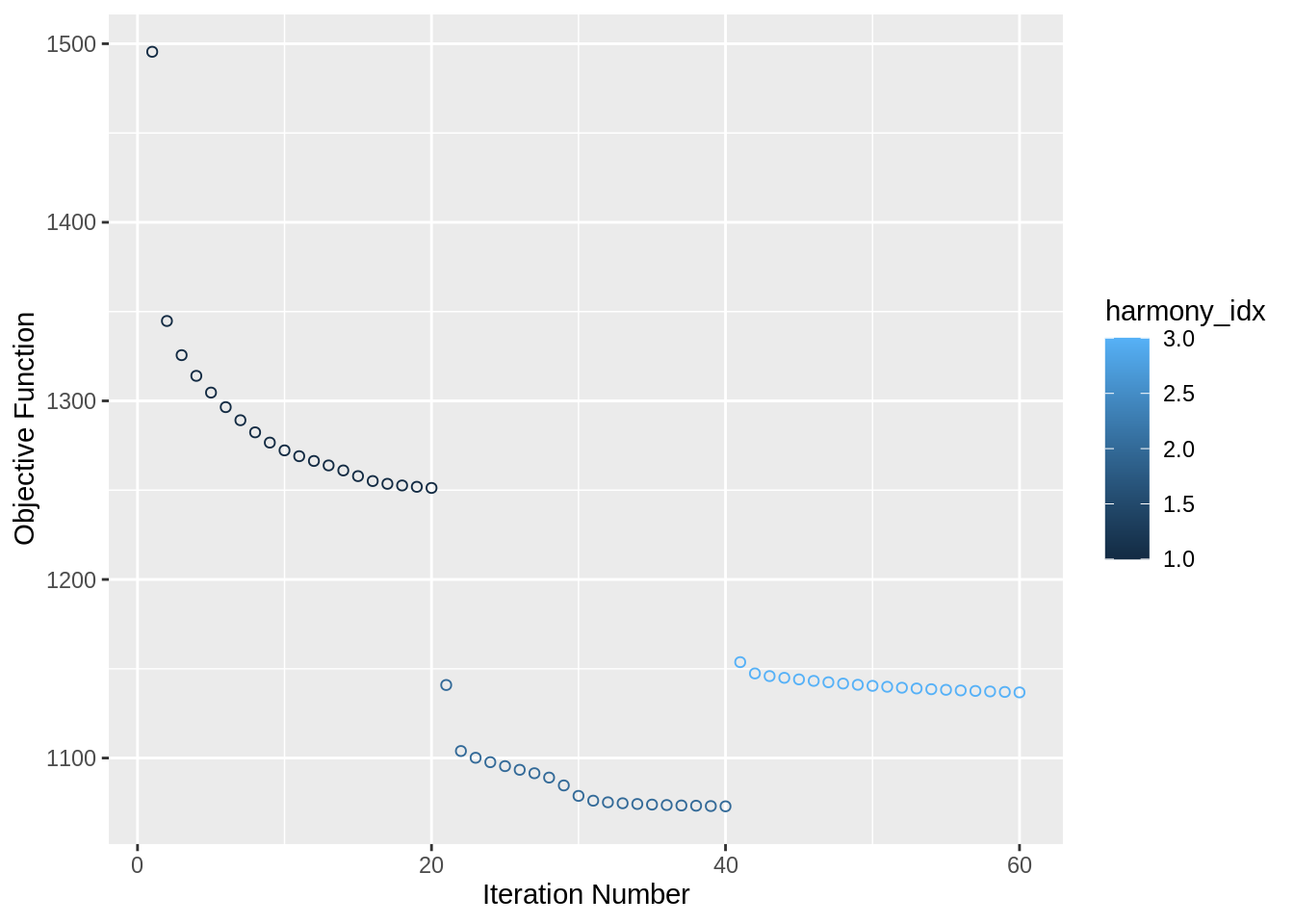
This generates the embeddings that we shall later use for all downstream analysis.
harmony_embeddings <- Embeddings(wb_harmony, 'harmony')
harmony_embeddings[1:5, 1:5]
## harmony_1 harmony_2 harmony_3 harmony_4 harmony_5
## AAACCCACATAACTCG-1 2.592137 -1.6045869 3.192993 -0.03594751 3.8447941
## AAACCCACATGTAACC-1 4.244764 3.2122684 -9.738222 -5.90380632 0.9607984
## AAACCCAGTGAGTCAG-1 3.208084 -2.1054920 2.035577 1.90984384 5.3665634
## AAACGAACAGTCAGTT-1 -1.106694 1.8151680 3.092745 -2.34038488 7.6785360
## AAACGAACATTCGGGC-1 4.735928 -0.4421468 -2.196355 2.77622970 -3.2385050Corrected PCA and distribution:
p1 <- DimPlot(object = wb_harmony, reduction = "harmony", pt.size = .1, group.by = "orig.ident") + NoLegend()
p2 <- VlnPlot(object = wb_harmony, features = "harmony_1", group.by = "orig.ident", pt.size = .1) + NoLegend()
plot_grid(p1,p2)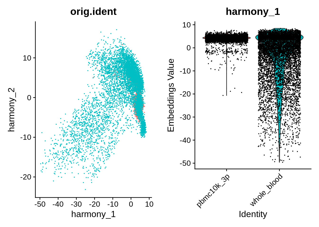
Run UMAP and perform Louvain clustering:
wb_harmony <- wb_harmony %>%
  RunUMAP(reduction = "harmony", dims = 1:30, verbose = F) %>%
  FindNeighbors(reduction = "harmony", k.param = 10, dims = 1:30) %>%
  FindClusters() %>%
  identity()
## Computing nearest neighbor graph## Computing SNN## Modularity Optimizer version 1.3.0 by Ludo Waltman and Nees Jan van Eck
##
## Number of nodes: 16421
## Number of edges: 266804
##
## Running Louvain algorithm...
## Maximum modularity in 10 random starts: 0.9230
## Number of communities: 31
## Elapsed time: 2 seconds## 1 singletons identified. 30 final clusters.wb_harmony <- SetIdent(wb_harmony,value = "orig.ident")
DimPlot(wb_harmony,reduction = "umap") + plot_annotation(title = "10k 3' PBMC and whole blood, after integration (Harmony)")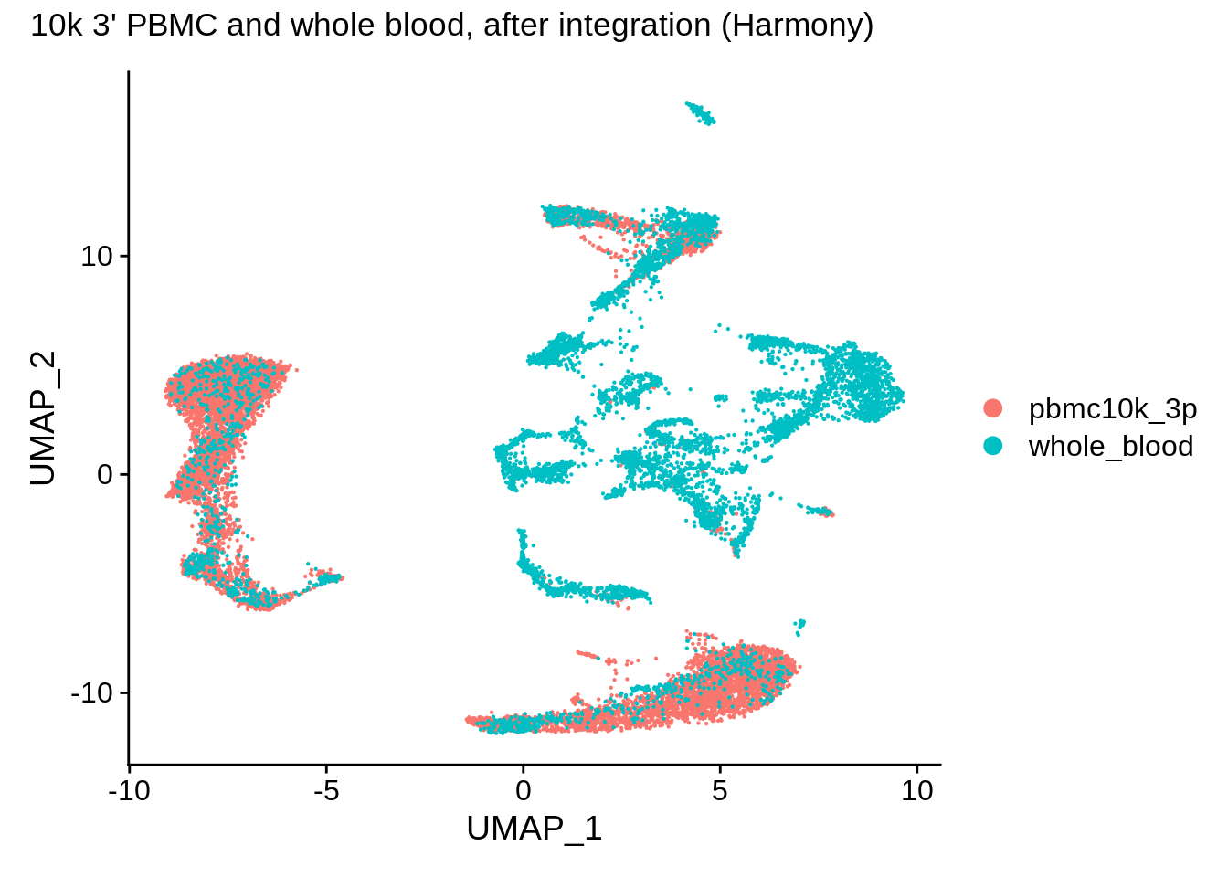
DimPlot(wb_harmony, reduction = "umap", group.by = "orig.ident", pt.size = .1, split.by = 'orig.ident') + NoLegend()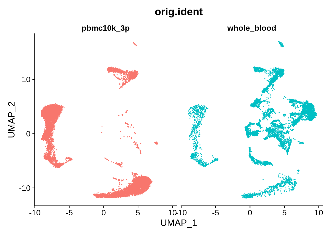
Corrected results for this dataset appear to be very similar to Seurat v3:
wb_harmony <- SetIdent(wb_harmony,value = "seurat_clusters")
DimPlot(wb_harmony,label = T) + NoLegend()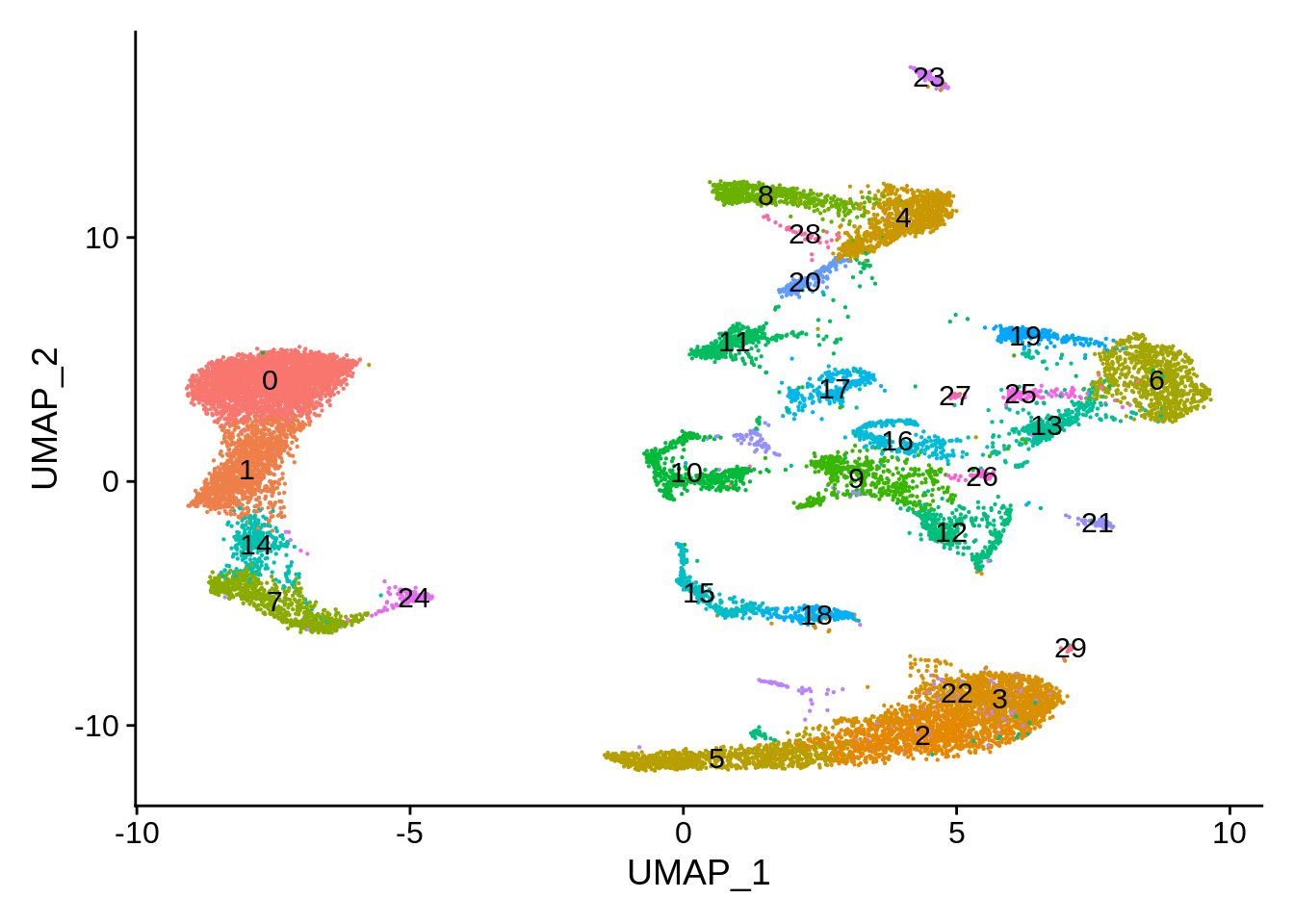
More detailed cluster examination also seems to confirm this:
plot_integrated_clusters(wb_harmony) ## Using cluster as id variables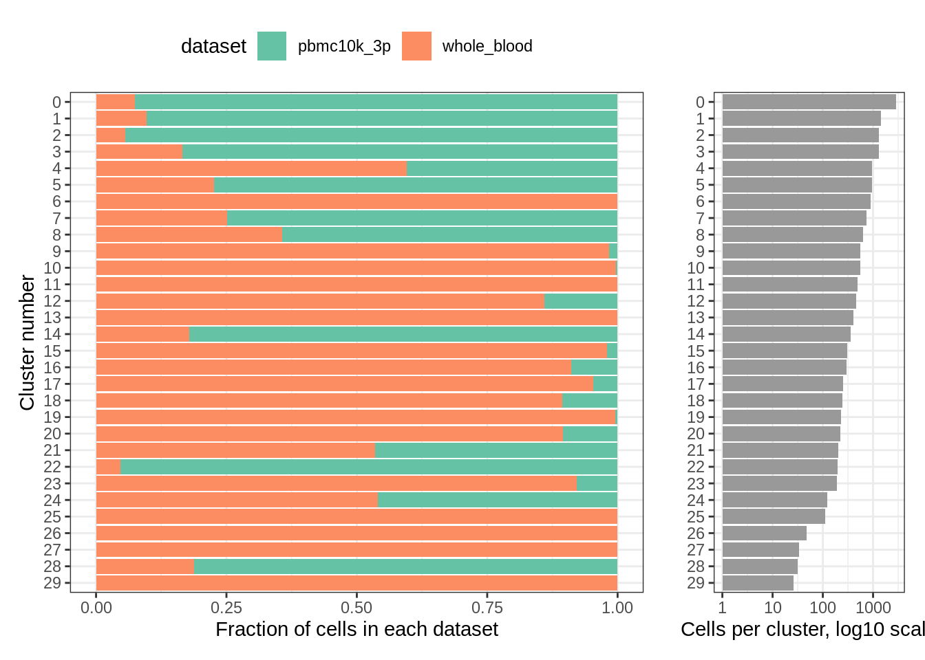
rm(wb_harmony)9.10 LIGER, 3’ 10k PBMC cells and whole blood STRT-Seq
Finally, let’s do data integration with LIGER. This step takes several minutes to run:
wb_liger    <- merge(srat_3p,srat_wb)

wb_liger    <- NormalizeData(wb_liger)
wb_liger    <- FindVariableFeatures(wb_liger)
wb_liger    <- ScaleData(wb_liger, split.by = "orig.ident", do.center = F)
## Scaling data matrix## Scaling data from split pbmc10k_3p## Scaling data from split whole_bloodwb_liger <- RunOptimizeALS(wb_liger, k = 30, lambda = 5, split.by = "orig.ident")##
|
| | 0%
|
|== | 3%
|
|===== | 7%
|
|======= | 10%
|
|========= | 13%
|
|============ | 17%
|
|============== | 20%
|
|================ | 23%
|
|=================== | 27%
|
|===================== | 30%
|
|======================= | 33%
|
|========================== | 37%
|
|============================ | 40%
|
|============================== | 43%
|
|================================= | 47%
|
|=================================== | 50%
|
|===================================== | 53%
|
|======================================== | 57%
|
|========================================== | 60%
|
|============================================ | 63%
|
|=============================================== | 67%
|
|================================================= | 70%
|
|=================================================== | 73%
|
|====================================================== | 77%
|
|======================================================== | 80%
|
|========================================================== | 83%
|
|============================================================= | 87%
|
|=============================================================== | 90%
|
|================================================================= | 93%
|
|==================================================================== | 97%
|
|======================================================================| 100%
## Finished in 8.023508 mins, 30 iterations.
## Max iterations set: 30.
## Final objective delta: 7.198128e-05.
## Best results with seed 1.## Warning: No columnames present in cell embeddings, setting to 'riNMF_1:30'wb_liger <- RunQuantileNorm(wb_liger, split.by = "orig.ident")We will then perform Louvain clustering (FindNeighbors and FindClusters) with the settings similar to what we have been using before:
wb_liger <- FindNeighbors(wb_liger,reduction = "iNMF",k.param = 10,dims = 1:30)## Computing nearest neighbor graph## Computing SNNwb_liger <- FindClusters(wb_liger)## Modularity Optimizer version 1.3.0 by Ludo Waltman and Nees Jan van Eck
##
## Number of nodes: 16421
## Number of edges: 267813
##
## Running Louvain algorithm...
## Maximum modularity in 10 random starts: 0.9197
## Number of communities: 35
## Elapsed time: 1 secondsLet’s look at the corrected UMAP plot in a couple of different ways:
wb_liger    <- RunUMAP(wb_liger, dims = 1:ncol(wb_liger[["iNMF"]]), reduction = "iNMF",verbose = F)
wb_liger <- SetIdent(wb_liger,value = "orig.ident")
DimPlot(wb_liger,reduction = "umap") + plot_annotation(title = "10k 3' PBMC and 10k 5' PBMC cells, after integration (LIGER)")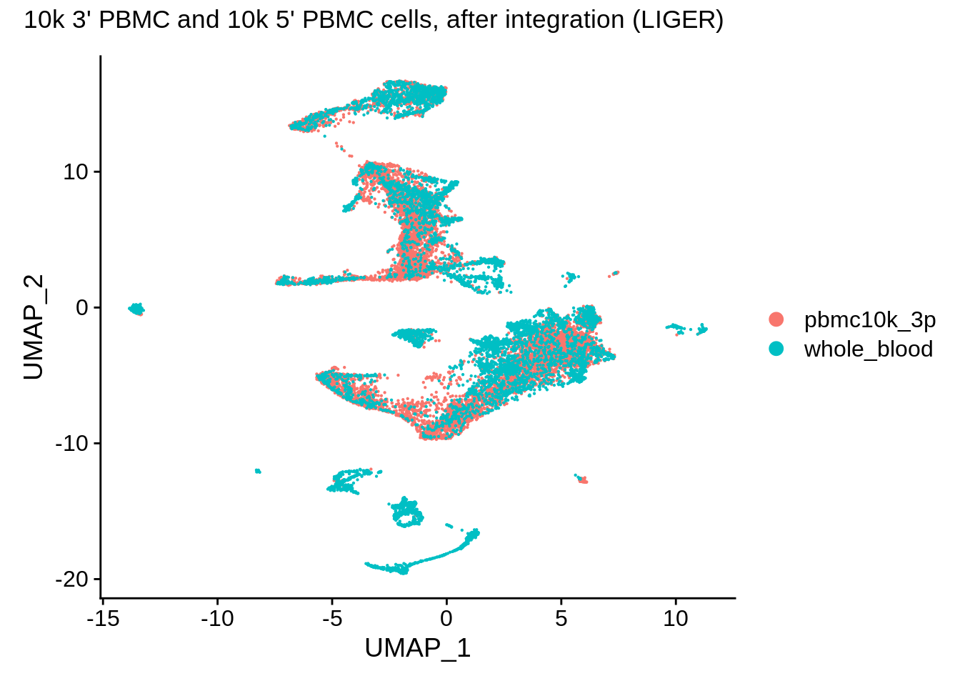
DimPlot(wb_liger, reduction = "umap", group.by = "orig.ident", pt.size = .1, split.by = 'orig.ident') + NoLegend()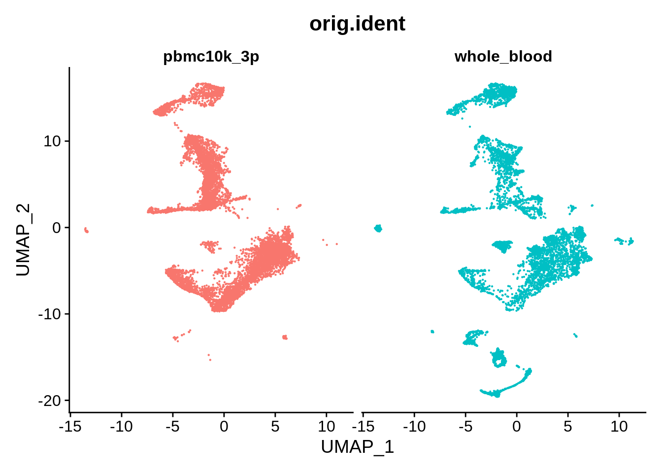
Finally, a look at distribution of datasets per cluster:
plot_integrated_clusters(wb_liger)## Using cluster as id variables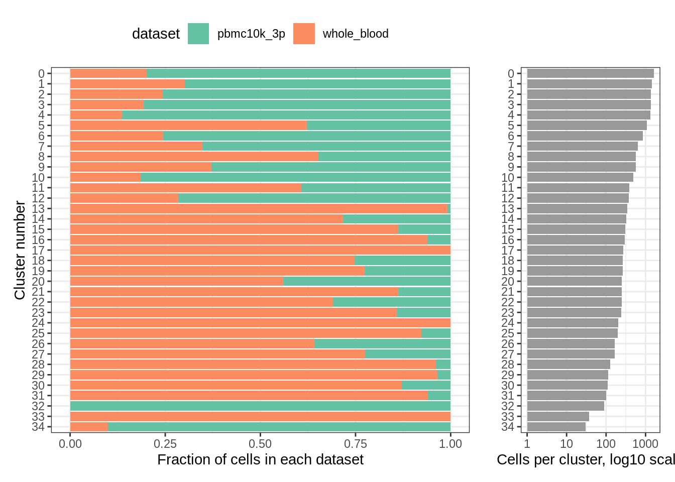
rm(wb_liger)
rm(srat_wb)
rm(srat_3p)
9.10.1 sessionInfo()
View session info
## R version 4.2.1 (2022-06-23)
## Platform: x86_64-pc-linux-gnu (64-bit)
## Running under: Ubuntu 20.04.2 LTS
##
## Matrix products: default
## BLAS:   /usr/lib/x86_64-linux-gnu/blas/libblas.so.3.9.0
## LAPACK: /usr/lib/x86_64-linux-gnu/lapack/liblapack.so.3.9.0
##
## locale:
##  [1] LC_CTYPE=en_US.UTF-8       LC_NUMERIC=C
##  [3] LC_TIME=en_US.UTF-8        LC_COLLATE=en_US.UTF-8
##  [5] LC_MONETARY=en_US.UTF-8    LC_MESSAGES=en_US.UTF-8
##  [7] LC_PAPER=en_US.UTF-8       LC_NAME=C
##  [9] LC_ADDRESS=C               LC_TELEPHONE=C
## [11] LC_MEASUREMENT=en_US.UTF-8 LC_IDENTIFICATION=C
##
## attached base packages:
## [1] stats     graphics  grDevices utils     datasets  methods   base
##
## other attached packages:
##  [1] ggplot2_3.3.6         dplyr_1.0.9           RColorBrewer_1.1-3
##  [4] reshape2_1.4.4        rliger_1.0.0          Matrix_1.4-1
##  [7] cowplot_1.1.1         harmony_0.1.0         Rcpp_1.0.9
## [10] patchwork_1.1.1       SeuratWrappers_0.3.0  SeuratDisk_0.0.0.9020
## [13] sp_1.5-0              SeuratObject_4.1.0    Seurat_4.1.1
## [16] knitr_1.39
##
## loaded via a namespace (and not attached):
##   [1] plyr_1.8.7            igraph_1.3.2          lazyeval_0.2.2
##   [4] splines_4.2.1         listenv_0.8.0         scattermore_0.8
##   [7] digest_0.6.29         foreach_1.5.2         htmltools_0.5.2
##  [10] fansi_1.0.3           magrittr_2.0.3        tensor_1.5
##  [13] cluster_2.1.3         doParallel_1.0.17     ROCR_1.0-11
##  [16] remotes_2.4.2         globals_0.15.1        matrixStats_0.62.0
##  [19] R.utils_2.12.0        spatstat.sparse_2.1-1 colorspace_2.0-3
##  [22] ggrepel_0.9.1         xfun_0.31             crayon_1.5.1
##  [25] jsonlite_1.8.0        progressr_0.10.1      spatstat.data_2.2-0
##  [28] survival_3.3-1        zoo_1.8-10            iterators_1.0.14
##  [31] glue_1.6.2            polyclip_1.10-0       gtable_0.3.0
##  [34] leiden_0.4.2          future.apply_1.9.0    abind_1.4-5
##  [37] scales_1.2.0          DBI_1.1.3             spatstat.random_2.2-0
##  [40] miniUI_0.1.1.1        riverplot_0.10        viridisLite_0.4.0
##  [43] xtable_1.8-4          reticulate_1.25       spatstat.core_2.4-4
##  [46] mclust_5.4.10         bit_4.0.4             rsvd_1.0.5
##  [49] htmlwidgets_1.5.4     httr_1.4.3            FNN_1.1.3.1
##  [52] ellipsis_0.3.2        ica_1.0-3             farver_2.1.1
##  [55] pkgconfig_2.0.3       R.methodsS3_1.8.2     sass_0.4.1
##  [58] uwot_0.1.11           deldir_1.0-6          utf8_1.2.2
##  [61] labeling_0.4.2        tidyselect_1.1.2      rlang_1.0.4
##  [64] later_1.3.0           munsell_0.5.0         tools_4.2.1
##  [67] cli_3.3.0             generics_0.1.3        ggridges_0.5.3
##  [70] evaluate_0.15         stringr_1.4.0         fastmap_1.1.0
##  [73] yaml_2.3.5            goftest_1.2-3         bit64_4.0.5
##  [76] fitdistrplus_1.1-8    purrr_0.3.4           RANN_2.6.1
##  [79] pbapply_1.5-0         future_1.26.1         nlme_3.1-157
##  [82] mime_0.12             ggrastr_1.0.1         R.oo_1.25.0
##  [85] hdf5r_1.3.5           compiler_4.2.1        beeswarm_0.4.0
##  [88] plotly_4.10.0         png_0.1-7             spatstat.utils_2.3-1
##  [91] tibble_3.1.7          bslib_0.3.1           stringi_1.7.8
##  [94] highr_0.9             RSpectra_0.16-1       rgeos_0.5-9
##  [97] lattice_0.20-45       vctrs_0.4.1           pillar_1.7.0
## [100] lifecycle_1.0.1       BiocManager_1.30.18   spatstat.geom_2.4-0
## [103] lmtest_0.9-40         jquerylib_0.1.4       RcppAnnoy_0.0.19
## [106] data.table_1.14.2     irlba_2.3.5           httpuv_1.6.5
## [109] R6_2.5.1              bookdown_0.27         promises_1.2.0.1
## [112] KernSmooth_2.23-20    gridExtra_2.3         vipor_0.4.5
## [115] parallelly_1.32.0     codetools_0.2-18      MASS_7.3-58
## [118] assertthat_0.2.1      withr_2.5.0           sctransform_0.3.3
## [121] mgcv_1.8-40           parallel_4.2.1        grid_4.2.1
## [124] rpart_4.1.16          tidyr_1.2.0           rmarkdown_2.14
## [127] Rtsne_0.16            shiny_1.7.1           ggbeeswarm_0.6.0