5 scRNA-seq Analysis with Bioconductor

QUESTIONS

How can I import single-cell data into R?
How are different types of data/information (e.g. cell information, gene information, etc.) stored and manipulated?
How can I obtain basic summary metrics for cells and genes and filter the data accordingly?
How can I visually explore these metrics?

LEARNING OBJECTIVES

Understand how single-cell data is stored in the Bioconductor SingleCellExperiment object.
Create a SingleCellExperiment object from processed scRNA-seq count data.
Access the different parts of a SingleCellExperiment object, such as rowData, colData and assay.
Obtain several summary metrics from a matrix, to summarise information across cells or genes.
Apply basic filters to the data, by constructing logical vectors and subset the object using the [ operator.
Produce basic data visualisations directly fron the data stored in the SingleCellExperiment object.

In this chapter we will start our practical introduction of the core packages used in our analysis.

We will use a dataset of induced pluripotent stem cells generated from three different individuals (Tung et al. 2017) in Yoav Gilad’s lab at the University of Chicago. The experiments were carried out on the Fluidigm C1 platform using unique molecular identifiers (UMIs) for quantification. The data files are located in the data/tung folder in your working directory. The original file can be found on the public NCBI repository GEO accession GSE77288 (file named: GSE77288_molecules-raw-single-per-sample.txt.gz).

NOTE:

A couple of things that are missing from these materials:

sparse matrix. Because it’s using the tung dataset, we just get a regular matrix. If we decide to use a 10x dataset instead, it might be easier to introduce that as well.
rowData - I didn’t include any gene annotation, although we could easily include that as well, for example with information about which genes are nuclear or mitochondrial.

5.1 Packages for scRNA-seq Analysis

There are several possible software packages (or package “ecosystems”) that can be used for single-cell analysis. In this course we’re going to focus on a collection of packages that are part of the Bioconductor project.

Bioconductor is a repository of R packages specifically developed for biological analyses. It has an excellent collection of packages for scRNA-seq analysis, which are summarised in the Orchestrating Single-Cell Analysis with Bioconductor book. The advantage of Bioconductor is that it has strict requirements for package submission, including installation on every platform and full documentation with a tutorial (called a vignette) explaining how the package should be used. Bioconductor also encourages utilization of standard data structures/classes and coding style/naming conventions, so that, in theory, packages and analyses can be combined into large pipelines or workflows. For scRNA-seq specifically, the standard data object used is called SingleCellExperiment, which we will learn more about in this section.

Seurat is another popular R package that uses its own data object called Seurat. The Seurat package includes a very large collection of functions and excellent documentation. Because of its popularity, several other packages nowadays are also compatible with the Seurat object. Although not the main focus of this course, we have a section illustrating an analysis workflow using this package: Analysis of scRNA-seq with Seurat.

Scanpy is a popular python package for scRNA-seq analysis, which stores data in an object called AnnData (annotated data). Similarly to Seurat and Bioconductor, developers can write extensions to the main package compatible with the AnnData package, allowing the community to expand on the functionality.

Although our main focus is on Bioconductor packages, the concepts we will learn about throughout this course should apply to the other alternatives, the main thing that changes is the exact syntax used.

5.2 The `SingleCellExperiment` Object

Expression data is usually stored as a feature-by-sample matrix of expression quantification. In scRNA-seq analysis we typically start our analysis from a matrix of counts, representing the number of reads/UMIs that aligned to a particular feature for each cell. Features can be things like genes, isoforms or exons. Usually, analyses are done at the gene-level, and that is what we will focus on in this course.

Besides our quantification matrix, we may also have information about each gene (e.g. their genome location, which type of gene they are, their length, etc.) and information about our cells (e.g. their tissue of origin, patient donor, processing batch, disease status, treatment exposure, etc.).

We may also produce other matrices from our raw count data, for example a matrix of normalised counts. And finally, because single-cell experiment data is very high dimensional (with thousands of cells and thousands of genes), we often employ dimensionality reduction techniques to capture the main variation in the data at lower dimensions.

SingleCellExperiment (SCE for short) is an object that stores all this information in a synchronised manner. The different parts of the object can be access by special functions:

One or more matrices of expression can be accessed by functions assay or assays
Information about the genes (the rows of the object) can be obtained using rowData function.
Information about the cells (the columns of the object) can be accessed by function colData.

Some of these data are stored in the slots with similar names and can be accessed by @ operator, but usage of accessor functions is consedered as a better programming style.

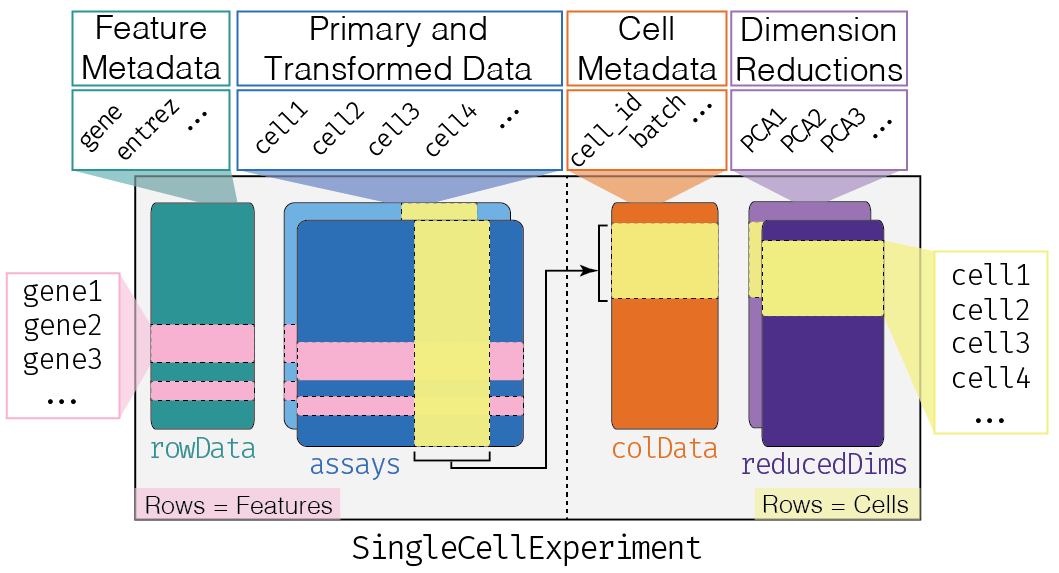
The SingleCellExperiment object. Features (e.g. genes, isoforms or exons) are stored as rows and their metadata is in a rowData slot. Cells are stored as columns, with their metadata in colData slot. Matrices of expression are stored in the assay slots. Dimensionality reduction projections of the cells are stored in the reducedDim slots.

5.2.1 Creating SCE Objects

Let’s start by creating a SingleCellExperiment object from our data. We have two files in data/tung:

counts.txt - a tab-delimited text file with the gene counts for each gene/cell.
annotation.txt - a tab-delimited text file with the cell annotations.

Let’s read these into R, using the standard read.table() function:

tung_counts <- read.table("data/tung/molecules.txt", sep = "\t")
tung_annotation <- read.table("data/tung/annotation.txt", sep = "\t", header = TRUE)

We can now create a SingleCellExperiment object using the function of the same name:

# load the library
library(SingleCellExperiment)

# note that the data passed to the assay slot has to be a matrix!
tung <- SingleCellExperiment(
  assays = list(counts = as.matrix(tung_counts)),
  colData = tung_annotation
)

# remove the original tables as we don't need them anymore
rm(tung_counts, tung_annotation)

If we print the contents of this object, we will get several useful pieces of information:

tung

## class: SingleCellExperiment 
## dim: 19027 864 
## metadata(0):
## assays(1): counts
## rownames(19027): ENSG00000237683 ENSG00000187634 ... ERCC-00170
##   ERCC-00171
## rowData names(0):
## colnames(864): NA19098.r1.A01 NA19098.r1.A02 ... NA19239.r3.H11
##   NA19239.r3.H12
## colData names(5): individual replicate well batch sample_id
## reducedDimNames(0):
## mainExpName: NULL
## altExpNames(0):

We have 19027 genes (rows) and 864 cells (columns).
There is a single assay named “counts.”
We can preview some of the gene names (“rownames”) and cell names (“colnames”).
There is no gene metadata (“rowData” is empty).
We can see some of the metadata for cells is (“colData names”).

To access different parts of the SCE object, we can use the following accessor functions:

Function	Description
`rowData(sce)`	Table of gene metadata.
`colData(sce)`	Table of cell metadata.
`assay(sce, "counts")`	The assay named “counts.”
`reducedDim(sce, "PCA")`	The reduced dimensionality table named “PCA”
`sce$colname`	Shortcut to access the colum “colname” from `colData`. This is equivalent to `colData(sce)$colname`
`sce[<rows>, <columns>]`	We can use the square brackets to subset the SCE object by rows or columns, similarly to how we subset `matrix` or `data.frame` objects

Naming Assays

Assays can have any name we wish. However, there are some conventions we can follow:

counts: Raw count data, e.g. number of reads or transcripts for a particular gene.
normcounts: Normalized values on the same scale as the original counts. For example, counts divided by cell-specific size factors that are centred at unity.
logcounts: Log-transformed counts or count-like values. In most cases, this will be defined as log-transformed normcounts, e.g. using log base 2 and a pseudo-count of 1.
cpm: Counts-per-million. This is the read count for each gene in each cell, divided by the library size of each cell in millions.
tpm: Transcripts-per-million. This is the number of transcripts for each gene in each cell, divided by the total number of transcripts in that cell (in millions).

Each of these has a function, so that we can access the “counts” assay using the counts() function. Therefore, these two are equivalent:

counts(tung)
assay(tung, "counts")

Creating SingleCellExperiment objects like we did above should work for any use case, as long as we have a matrix of counts that we can read to a file. However, to read the output of the popular tool cellranger (used to quantify 10x Chromium data), there is a dedicated function in the DropletUtils package, which simplifies the process of importing the data. Here is an example usage:

library(DropletUtils)

# importing the raw count data
sce <- read10xCounts("data/pbmc_1k_raw")

# importing the pre-filtered count data
sce <- read10xCounts("data/pbmc_1k_filtered")

Exercise 1

What are the classes of the “colData” and “assay” slots of our tung object?

Hint
To check the class of an object you can use the class() function.
How many batches and cells per batch are there? Does that number make sense?

Hint
You can tabulate the values in a column from a data.frame using table(x$column_name)

Answer

A1.

Checking the class of the “colData” slot:

class(colData(tung))

## [1] "DFrame"
## attr(,"package")
## [1] "S4Vectors"

This is a DFrame object, which is a type of data.frame used in Bioconductor (in practice it can be used in the same way as a regular data.frame).

The “assay” slot is of class “matrix”:

class(counts(tung)) # or: class(assay(sce, "counts"))

## [1] "matrix" "array"

A2.

The information about cells is stored in the colData slot of our object:

colData(tung)

## DataFrame with 864 rows and 5 columns
##                 individual   replicate        well       batch      sample_id
##                <character> <character> <character> <character>    <character>
## NA19098.r1.A01     NA19098          r1         A01  NA19098.r1 NA19098.r1.A01
## NA19098.r1.A02     NA19098          r1         A02  NA19098.r1 NA19098.r1.A02
## NA19098.r1.A03     NA19098          r1         A03  NA19098.r1 NA19098.r1.A03
## NA19098.r1.A04     NA19098          r1         A04  NA19098.r1 NA19098.r1.A04
## NA19098.r1.A05     NA19098          r1         A05  NA19098.r1 NA19098.r1.A05
## ...                    ...         ...         ...         ...            ...
## NA19239.r3.H08     NA19239          r3         H08  NA19239.r3 NA19239.r3.H08
## NA19239.r3.H09     NA19239          r3         H09  NA19239.r3 NA19239.r3.H09
## NA19239.r3.H10     NA19239          r3         H10  NA19239.r3 NA19239.r3.H10
## NA19239.r3.H11     NA19239          r3         H11  NA19239.r3 NA19239.r3.H11
## NA19239.r3.H12     NA19239          r3         H12  NA19239.r3 NA19239.r3.H12

We can see that there is a column called “batch,” which is what we’re interested in looking at. To access columns from a data frame we can use $, so colData(tung)$batch would return a vector with all the values in that column of the data frame. There is also a short-cut to access these columns directly: tung$batch (without the need to use the colData() function first).

Now that we know how to access the column of our colData, we can use the table() function to check how many cells we have per batch:

table(tung$batch)

## 
## NA19098.r1 NA19098.r2 NA19098.r3 NA19101.r1 NA19101.r2 NA19101.r3 NA19239.r1 
##         96         96         96         96         96         96         96 
## NA19239.r2 NA19239.r3 
##         96         96

We can see that there are 96 cells in each of 9 batches. This number of cells per batch suggests that the protocol was done on 96-well plates, so the authors used a low-throughput method for their experiment.

5.2.2 Modifying SCE Objects

To modify parts of our SCE object we can use the <- assignment operator, together with the part of the object we wish to modify. For example, to create a new assay: assay(sce, "name_of_new_assay") <- new_matrix. Other use cases are summarised in the table below.

As an example, let’s create a simple transformation of our count data, by taking the log base 2 with an added pseudocount of 1 (otherwise log(0) = -Inf):

assay(tung, "logcounts") <- log2(counts(tung) + 1)

Because we named our assay “logcounts,” and this is one of the conventional assay names, we can use the dedicated function to access it:

# first 10 rows and 4 columns of the logcounts assay
logcounts(tung)[1:10, 1:4] # or: assay(tung, "logcounts")[1:10, 1:5]

##                 NA19098.r1.A01 NA19098.r1.A02 NA19098.r1.A03 NA19098.r1.A04
## ENSG00000237683       0.000000       0.000000       0.000000              1
## ENSG00000187634       0.000000       0.000000       0.000000              0
## ENSG00000188976       2.000000       2.807355       1.000000              2
## ENSG00000187961       0.000000       0.000000       0.000000              0
## ENSG00000187583       0.000000       0.000000       0.000000              0
## ENSG00000187642       0.000000       0.000000       0.000000              0
## ENSG00000188290       0.000000       0.000000       0.000000              0
## ENSG00000187608       1.000000       3.000000       0.000000              2
## ENSG00000188157       1.584963       2.000000       1.584963              2
## ENSG00000237330       0.000000       0.000000       0.000000              0

Here is a summary of other ways to modify data in SCE objects:

Code	Description
`assay(sce, "name") <- matrix`	Add a new assay matrix. The new matrix has to have matching rownames and colnames to the existing object.
`rowData(sce) <- data_frame`	Replace `rowData` with a new table (or add one if it does not exist).
`colData(sce) <- data_frame`	Replace `colData` with a new table (or add one if it does not exist).
`colData(sce)$column_name <- values`	Add a new column to the `colData` table (or replace it if it already exists).
`rowData(sce)$column_name <- values`	Add a new column to the `rowData` table (or replace it if it already exists).
`reducedDim(sce, "name") <- matrix`	Add a new dimensionality reduction matrix. The new matrix has to have matching colnames to the existing object.

5.2.3 Matrix Statistics

Because the main data stored in SingleCellExperiment objects is a matrix, it is useful to cover some functions that calculate summary metrics across rows or columns of a matrix. There are several functions to do this, detailed in the information box below.

For example, to calculate the mean counts per cell (columns) in our dataset:

colMeans(counts(tung))

We could add this information to our column metadata as a new column, which we could do as:

colData(tung)$mean_counts <- colMeans(counts(tung))

If we look at the colData slot we can see the new column has been added:

colData(tung)

## DataFrame with 864 rows and 6 columns
##                 individual   replicate        well       batch      sample_id
##                <character> <character> <character> <character>    <character>
## NA19098.r1.A01     NA19098          r1         A01  NA19098.r1 NA19098.r1.A01
## NA19098.r1.A02     NA19098          r1         A02  NA19098.r1 NA19098.r1.A02
## NA19098.r1.A03     NA19098          r1         A03  NA19098.r1 NA19098.r1.A03
## NA19098.r1.A04     NA19098          r1         A04  NA19098.r1 NA19098.r1.A04
## NA19098.r1.A05     NA19098          r1         A05  NA19098.r1 NA19098.r1.A05
## ...                    ...         ...         ...         ...            ...
## NA19239.r3.H08     NA19239          r3         H08  NA19239.r3 NA19239.r3.H08
## NA19239.r3.H09     NA19239          r3         H09  NA19239.r3 NA19239.r3.H09
## NA19239.r3.H10     NA19239          r3         H10  NA19239.r3 NA19239.r3.H10
## NA19239.r3.H11     NA19239          r3         H11  NA19239.r3 NA19239.r3.H11
## NA19239.r3.H12     NA19239          r3         H12  NA19239.r3 NA19239.r3.H12
##                mean_counts
##                  <numeric>
## NA19098.r1.A01     3.32801
## NA19098.r1.A02     3.36238
## NA19098.r1.A03     2.29306
## NA19098.r1.A04     2.83397
## NA19098.r1.A05     3.72560
## ...                    ...
## NA19239.r3.H08    3.097861
## NA19239.r3.H09    2.933568
## NA19239.r3.H10    0.316813
## NA19239.r3.H11    2.678615
## NA19239.r3.H12    4.068482

There are several functions that can be used to calculate summary metrics - such as mean, median, variance, etc. - across rows or columns of a matrix (or a sparse matrix).

Here are some of the functions available:

# row (feature) summaries
rowSums(counts(tung))  # sum
rowMeans(counts(tung)) # mean
rowSds(counts(tung))   # standard deviation
rowVars(counts(tung))  # variance
rowIQRs(counts(tung))  # inter-quartile range
rowMads(counts(tung))  # mean absolute deviation

# column (sample) summaries
colSums(counts(tung))  # sum
colMeans(counts(tung)) # mean
colSds(counts(tung))   # standard deviation
colVars(counts(tung))  # variance
colIQRs(counts(tung))  # inter-quartile range
colMads(counts(tung))  # mean absolute deviation

Exercise 2

Add a new column to colData named “total_counts” with the sum of counts in each cell.
Create a new assay called “cpm” (Counts-Per-Million), which contains the result of dividing the counts matrix by the total counts in millions.
How can you access this new assay?

Answer

A1.

Because we want the total counts per cell, and cells are stored as columns in the SCE object, we need to use the colSums() function:

colData(tung)$total_counts <- colSums(counts(tung))

A2.

We need to divide our counts matrix by the new column we’ve just created. Function sweep can be used to make it columnwise:

# function sweep takes following arguments:
# matrix to normalize
# dimention to normalize along (1 - by rows, 2 - by columns)
# statistics to normalize by
# function to use for normalization
assay(tung, "cpm") <- sweep(counts(tung),2,tung$total_counts/1e6,'/')
# check that column sums are 1e6 now
colSums(cpm(tung))[1:10]

## NA19098.r1.A01 NA19098.r1.A02 NA19098.r1.A03 NA19098.r1.A04 NA19098.r1.A05 
##          1e+06          1e+06          1e+06          1e+06          1e+06 
## NA19098.r1.A06 NA19098.r1.A07 NA19098.r1.A08 NA19098.r1.A09 NA19098.r1.A10 
##          1e+06          1e+06          1e+06          1e+06          1e+06

We also divided by 1e6, so that it’s in units of millions.

Note that we’re dividing a matrix (counts(tung)) by a vector (tung$total_counts). R will do this division row-by-row, and “recycles” the tung$total_counts vector each time it starts a new rown of the counts(tung) matrix.

A3.

Because “cpm” is one of the conventional names used for an assay, we can access it with the cpm() function:

# these two are equivalent
cpm(tung)
assay(tung, "cpm")

5.2.4 Subsetting SCE Objects

Similarly to the standard data.frame and matrix objects in R, we can use the [ operator to subset our SingleCellExperiment either by rows (genes) or columns (cells). The general syntax is: sce[rows_of_interest, columns_of_interest].

For example:

# subset by numeric index
tung[1:3, ] # the first 3 genes, keep all cells
tung[, 1:3] # the first 3 cells, keep all genes
tung[1:3, 1:2] # the first 3 genes and first 2 cells

# subset by name
tung[c("ENSG00000069712", "ENSG00000237763"), ]
tung[, c("NA19098.r1.A01", "NA19098.r1.A03")]
tung[c("ENSG00000069712", "ENSG00000237763"), c("NA19098.r1.A01", "NA19098.r1.A03")]

Although manually subsetting the object can sometimes be useful, more often we want to do conditional subsetting based on TRUE/FALSE logical statements. This is extremely useful for filtering our data. Let see some practical examples.

Let’s say we wanted to retain genes with a mean count greater than 0.01. As we saw, to calculate the mean counts per gene (rows in the SCE object), we can use the rowMeans() function:

# calculate the mean counts per gene
gene_means <- rowMeans(counts(tung))

# print the first 10 values
gene_means[1:10]

## ENSG00000237683 ENSG00000187634 ENSG00000188976 ENSG00000187961 ENSG00000187583 
##      0.28240741      0.03009259      2.63888889      0.23842593      0.01157407 
## ENSG00000187642 ENSG00000188290 ENSG00000187608 ENSG00000188157 ENSG00000237330 
##      0.01273148      0.02430556      1.89583333      3.32523148      0.02199074

We can turn this into a TRUE/FALSE vector by using a logical operator:

gene_means[1:10] > 0.01

## ENSG00000237683 ENSG00000187634 ENSG00000188976 ENSG00000187961 ENSG00000187583 
##            TRUE            TRUE            TRUE            TRUE            TRUE 
## ENSG00000187642 ENSG00000188290 ENSG00000187608 ENSG00000188157 ENSG00000237330 
##            TRUE            TRUE            TRUE            TRUE            TRUE

We can use such a logical vector inside [ to filter our data, which will return only the cases where the value is TRUE:

tung[gene_means > 0.01, ]

## class: SingleCellExperiment 
## dim: 16052 864 
## metadata(0):
## assays(3): counts logcounts cpm
## rownames(16052): ENSG00000237683 ENSG00000187634 ... ERCC-00170
##   ERCC-00171
## rowData names(0):
## colnames(864): NA19098.r1.A01 NA19098.r1.A02 ... NA19239.r3.H11
##   NA19239.r3.H12
## colData names(7): individual replicate ... mean_counts total_counts
## reducedDimNames(0):
## mainExpName: NULL
## altExpNames(0):

Notice how the resulting SCE object has fewer genes than the original.

Another common use case is to retain cells with a certain number of genes above a certain threshold of expression. For this question, we need to break the problem into parts. First let’s check in our counts matrix, which genes are expressed above a certain threshold:

# counts of at least 1
counts(tung) > 0

##                 NA19098.r1.A01 NA19098.r1.A02 NA19098.r1.A03 NA19098.r1.A04
## ENSG00000237683          FALSE          FALSE          FALSE           TRUE
## ENSG00000187634          FALSE          FALSE          FALSE          FALSE
## ENSG00000188976           TRUE           TRUE           TRUE           TRUE
## ENSG00000187961          FALSE          FALSE          FALSE          FALSE
## ENSG00000187583          FALSE          FALSE          FALSE          FALSE
## ENSG00000187642          FALSE          FALSE          FALSE          FALSE
## ENSG00000188290          FALSE          FALSE          FALSE          FALSE
## ENSG00000187608           TRUE           TRUE          FALSE           TRUE
## ENSG00000188157           TRUE           TRUE           TRUE           TRUE
## ENSG00000237330          FALSE          FALSE          FALSE          FALSE

We can see that our matrix is now composed of only TRUE/FALSE values. Because TRUE/FALSE are encoded as 1/0, we can use colSums() to calculate the total number of genes above this threshold per cell:

# total number of detected genes per cell
total_detected_per_cell <- colSums(counts(tung) > 0)

# print the first 10 values
total_detected_per_cell[1:10]

## NA19098.r1.A01 NA19098.r1.A02 NA19098.r1.A03 NA19098.r1.A04 NA19098.r1.A05 
##           8368           8234           7289           7985           8619 
## NA19098.r1.A06 NA19098.r1.A07 NA19098.r1.A08 NA19098.r1.A09 NA19098.r1.A10 
##           8659           8054           9429           8243           9407

Finally, we can use this vector to apply our final condition, for example that we want cells with at least 5000 detected genes:

tung[, total_detected_per_cell > 5000]

## class: SingleCellExperiment 
## dim: 19027 849 
## metadata(0):
## assays(3): counts logcounts cpm
## rownames(19027): ENSG00000237683 ENSG00000187634 ... ERCC-00170
##   ERCC-00171
## rowData names(0):
## colnames(849): NA19098.r1.A01 NA19098.r1.A02 ... NA19239.r3.H11
##   NA19239.r3.H12
## colData names(7): individual replicate ... mean_counts total_counts
## reducedDimNames(0):
## mainExpName: NULL
## altExpNames(0):

Notice how the new SCE object has fewer cells than the original.

Here is a summary of the syntax used for some common filters:

Filter on	Code	Description
Cells	`colSums(counts(sce)) > x`	Total counts per cell greater than x.
Cells	`colSums(counts(sce) > x) > y`	Cells with at least y genes having counts greater than x.
Genes	`rowSums(counts(sce)) > x`	Total counts per gene greater than x.
Genes	`rowSums(counts(sce) > x) > y`	Genes with at least y cells having counts greater than x.

Exercise 3

Create a new object called tung_filtered which contains:
- cells with at least 25000 total counts
- genes that have more than 5 counts in at least half of the cells
How many cells and genes are you left with?

Answer

Let’s do this in parts, by creating a TRUE/FALSE logical vector for each condition. For the first condition, we need to calculate the total counts per cell (columns), and threshold it based on the values being greater than or equal to 25000:

cell_filter <- colSums(counts(tung)) >= 25000

# check how many TRUE/FALSE have
table(cell_filter)

## cell_filter
## FALSE  TRUE 
##    46   818

For the second condition, we need to apply two nested conditions. By consulting the table above, we can achieve this by:

gene_filter <- rowSums(counts(tung) > 5) > ncol(tung)/2

# check how many TRUE/FALSE have
table(gene_filter)

## gene_filter
## FALSE  TRUE 
## 16811  2216

Finally, we can use both of these logical vectors to subset our object:

tung_filtered <- tung[gene_filter, cell_filter]

tung_filtered

## class: SingleCellExperiment 
## dim: 2216 818 
## metadata(0):
## assays(3): counts logcounts cpm
## rownames(2216): ENSG00000175756 ENSG00000242485 ... ERCC-00145
##   ERCC-00171
## rowData names(0):
## colnames(818): NA19098.r1.A01 NA19098.r1.A02 ... NA19239.r3.H11
##   NA19239.r3.H12
## colData names(7): individual replicate ... mean_counts total_counts
## reducedDimNames(0):
## mainExpName: NULL
## altExpNames(0):

5.3 Visual Data Exploration

There are several ways to produce visualisations from our data. We will use the ggplot2 package for our plots, together with the Bioconductor package scater, which has some helper functions for retrieving data from a SingleCellExperiment object ready for visualisation.

As a reminder, the basic components of a ggplot are:

A data.frame with data to be plotted
The variables (columns of the data.frame) that will be mapped to different aesthetics of the graph (e.g. axis, colours, shapes, etc.)
the geometry that will be drawn on the graph (e.g. points, lines, boxplots, violinplots, etc.)

This translates into the following basic syntax:

ggplot(data = <data.frame>, 
       mapping = aes(x = <column of data.frame>, y = <column of data.frame>)) +
   geom_<type of geometry>()

For example, let’s visualise what the distribution of total counts per cell is for each of our batches. This information is stored in colData, so we need to extract it from our object and convert it to a standard data.frame:

cell_info <- as.data.frame(colData(tung))

head(cell_info)

##                individual replicate well      batch      sample_id mean_counts
## NA19098.r1.A01    NA19098        r1  A01 NA19098.r1 NA19098.r1.A01    3.328008
## NA19098.r1.A02    NA19098        r1  A02 NA19098.r1 NA19098.r1.A02    3.362380
## NA19098.r1.A03    NA19098        r1  A03 NA19098.r1 NA19098.r1.A03    2.293057
## NA19098.r1.A04    NA19098        r1  A04 NA19098.r1 NA19098.r1.A04    2.833973
## NA19098.r1.A05    NA19098        r1  A05 NA19098.r1 NA19098.r1.A05    3.725600
## NA19098.r1.A06    NA19098        r1  A06 NA19098.r1 NA19098.r1.A06    3.576549
##                total_counts
## NA19098.r1.A01        63322
## NA19098.r1.A02        63976
## NA19098.r1.A03        43630
## NA19098.r1.A04        53922
## NA19098.r1.A05        70887
## NA19098.r1.A06        68051

Now we are ready to make our plot:

# load the library
library(ggplot2)

ggplot(data = cell_info, aes(x = batch, y = total_counts)) +
  geom_violin(fill = 'brown') + theme_bw() + 
  theme(axis.text.x = element_text(angle = 45, vjust = 1, hjust=1))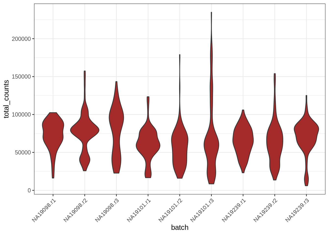

What if we wanted to visualise the distribution of expression of a particular gene in each batch? This now gets a little more complicated, because the gene expression information is stored in the counts assay of our SCE, whereas the batch information is in the colData. To bring both of these pieces of information together would require us to do a fair amount of data manipulation to put it all together into a single data.frame. This is where the scater package is very helpful, as it provides us with the ggcells() function that let’s us specify all these pieces of information for our plot.

For example, the same plot as above could have been done directly from our tung SCE object:

library(scater)

## Loading required package: scuttle

ggcells(tung, aes(x = batch, y = total_counts)) + 
  geom_violin(fill = 'orange') + theme_bw() + 
  theme(axis.text.x = element_text(angle = 45, vjust = 1, hjust=1))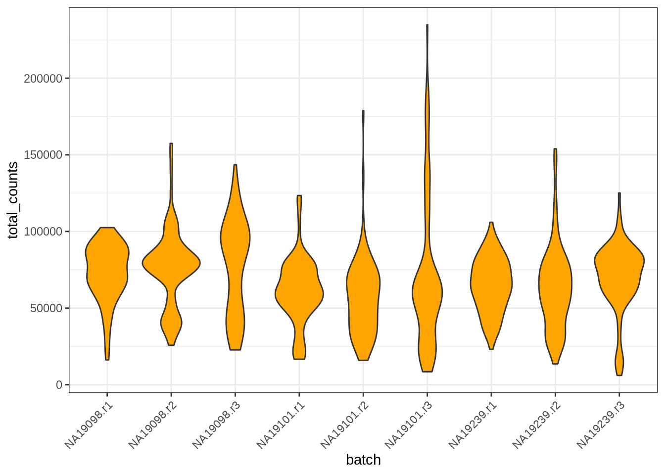

If we instead wanted to plot the expression for one of our genes, we could do it as:

library(scater)
ggcells(tung, aes(x = batch, y = ENSG00000198938), exprs_values = "logcounts") + 
  geom_violin(fill = 'coral2') + theme_bw() + 
  theme(axis.text.x = element_text(angle = 45, vjust = 1, hjust=1))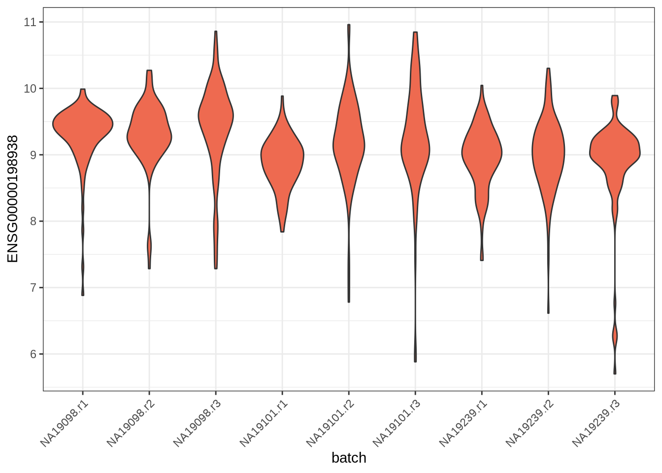

Note that we specified which assay we wanted to use for our expression values (exprs_values option). The default is “logcounts,” so we wouldn’t have had to specify it in this case, but it’s worth knowing that in case you want to visualise the expression from a different assay. The functionality provided by the scater package goes far beyond plotting, it also includes several functions for quality control, which we will return to in the next chapter.

Exercise 4

Make a scatterplot showing the relationship between the mean and the variance of the raw counts per cell. (Bonus: also colour the cells by batch.)

Hint

First create a new column in colData named “var_counts,” which contains the counts variance using the colVars() function.
Then use ggcells() to build a ggplot with “mean_counts” as the x-axis and “var_counts” as the y-axis.
You can use the geom_point() function to make a scatterplot.
Finally, to colour the points you can use the colour aesthetic.

What can you conclude from this data exploration, in terms of selecting highly variable genes for downstream analysis?

Answer

First we add a new column to colData, using the colVars() function to calculate variance of our counts for each cell (columns of the SCE object):

colData(tung)$var_counts <- colVars(counts(tung))

Now we are ready to make our plot, including using the colour aesthetic:

ggcells(tung, aes(mean_counts, var_counts)) +
  geom_point(aes(colour = batch)) + theme_bw()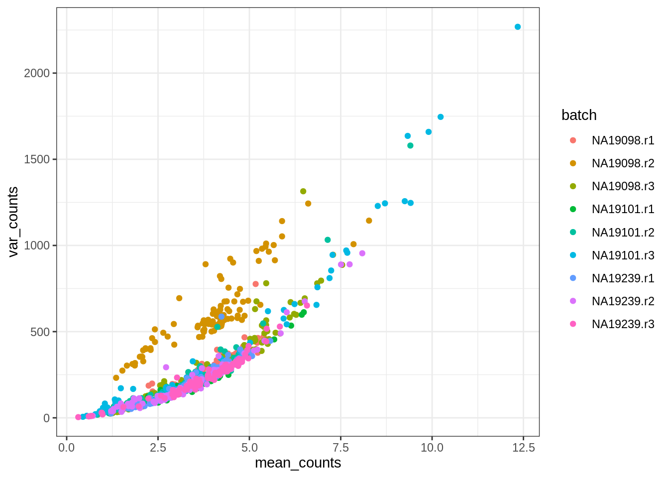

We can see that there is a positive correlation between the mean and variance of gene counts. This is a common feature of count data, in particular of RNA-seq data. Because of this relationship, it’s important to use tools that model the mean-variance relationship adequately, so that when we choose genes that are variable in our dataset, we’re not simply choosing genes that are more highly expressed.

5.4 Overview

KEY POINTS

The SingleCellExperiment (SCE) object is used to store expression data as well as information about our cells (columns) and genes (rows).
To create a new SCE object we can use the SingleCellExperiment() function. To read the output from cellranger we can use the dedicated function DropletUtils::read10xCounts().
The main parts of this object are:
- assay - one or more matrices of expression quantification.
  - There is one essential assay named “counts,” which contains the raw counts on which all other analyses are based on.
- rowData - information about our genes.
- colData - information about our cells.
- reducedDim - one or more reduced dimensionality representations of our data.
We can access all the parts of this object using functions of the same name. For example assay(sce, "counts") retrieves the counts matrix from the object.
We can add/modify parts of this object using the assignment operator <-. For example assay(sce, "logcounts") <- log2(counts(sce) + 1) would add a new assay named “logcounts” to our object.
Matrix summary metrics are very useful to explore the properties of our expression data. Some of the more useful functions include rowSums()/colSums() and rowMeans()/colMeans(). These can be used to summarise information from our assays, for example colSums(counts(sce)) would give us the total counts in each cell (columns).
Combining matrix summaries with conditional operators (>, <, ==, !=) can be used for conditional subsetting using [.
We can use the ggcells() function (from the scater package), to produce ggplot-style plots directly from our SCE object.

5.4.1 sessionInfo()

View session info

## R version 4.2.1 (2022-06-23)
## Platform: x86_64-pc-linux-gnu (64-bit)
## Running under: Ubuntu 20.04.2 LTS
## 
## Matrix products: default
## BLAS:   /usr/lib/x86_64-linux-gnu/blas/libblas.so.3.9.0
## LAPACK: /usr/lib/x86_64-linux-gnu/lapack/liblapack.so.3.9.0
## 
## locale:
##  [1] LC_CTYPE=en_US.UTF-8       LC_NUMERIC=C              
##  [3] LC_TIME=en_US.UTF-8        LC_COLLATE=en_US.UTF-8    
##  [5] LC_MONETARY=en_US.UTF-8    LC_MESSAGES=en_US.UTF-8   
##  [7] LC_PAPER=en_US.UTF-8       LC_NAME=C                 
##  [9] LC_ADDRESS=C               LC_TELEPHONE=C            
## [11] LC_MEASUREMENT=en_US.UTF-8 LC_IDENTIFICATION=C       
## 
## attached base packages:
## [1] stats4    stats     graphics  grDevices utils     datasets  methods  
## [8] base     
## 
## other attached packages:
##  [1] scater_1.24.0               scuttle_1.6.2              
##  [3] ggplot2_3.3.6               SingleCellExperiment_1.18.0
##  [5] SummarizedExperiment_1.26.1 Biobase_2.56.0             
##  [7] GenomicRanges_1.48.0        GenomeInfoDb_1.32.2        
##  [9] IRanges_2.30.0              S4Vectors_0.34.0           
## [11] BiocGenerics_0.42.0         MatrixGenerics_1.8.1       
## [13] matrixStats_0.62.0          knitr_1.39                 
## 
## loaded via a namespace (and not attached):
##  [1] viridis_0.6.2             sass_0.4.1               
##  [3] BiocSingular_1.12.0       viridisLite_0.4.0        
##  [5] jsonlite_1.8.0            DelayedMatrixStats_1.18.0
##  [7] bslib_0.3.1               assertthat_0.2.1         
##  [9] highr_0.9                 GenomeInfoDbData_1.2.8   
## [11] vipor_0.4.5               yaml_2.3.5               
## [13] ggrepel_0.9.1             pillar_1.7.0             
## [15] lattice_0.20-45           glue_1.6.2               
## [17] beachmat_2.12.0           digest_0.6.29            
## [19] XVector_0.36.0            colorspace_2.0-3         
## [21] htmltools_0.5.2           Matrix_1.4-1             
## [23] pkgconfig_2.0.3           bookdown_0.27            
## [25] zlibbioc_1.42.0           purrr_0.3.4              
## [27] scales_1.2.0              ScaledMatrix_1.4.0       
## [29] BiocParallel_1.30.3       tibble_3.1.7             
## [31] generics_0.1.3            farver_2.1.1             
## [33] ellipsis_0.3.2            withr_2.5.0              
## [35] cli_3.3.0                 magrittr_2.0.3           
## [37] crayon_1.5.1              evaluate_0.15            
## [39] fansi_1.0.3               beeswarm_0.4.0           
## [41] tools_4.2.1               lifecycle_1.0.1          
## [43] stringr_1.4.0             munsell_0.5.0            
## [45] DelayedArray_0.22.0       irlba_2.3.5              
## [47] compiler_4.2.1            jquerylib_0.1.4          
## [49] rsvd_1.0.5                rlang_1.0.4              
## [51] grid_4.2.1                RCurl_1.98-1.7           
## [53] BiocNeighbors_1.14.0      bitops_1.0-7             
## [55] labeling_0.4.2            rmarkdown_2.14           
## [57] gtable_0.3.0              codetools_0.2-18         
## [59] DBI_1.1.3                 R6_2.5.1                 
## [61] gridExtra_2.3             dplyr_1.0.9              
## [63] fastmap_1.1.0             utf8_1.2.2               
## [65] stringi_1.7.8             ggbeeswarm_0.6.0         
## [67] parallel_4.2.1            Rcpp_1.0.9               
## [69] vctrs_0.4.1               tidyselect_1.1.2         
## [71] xfun_0.31                 sparseMatrixStats_1.8.0

5 scRNA-seq Analysis with Bioconductor

5.1 Packages for scRNA-seq Analysis

5.2 The SingleCellExperiment Object

5.2.1 Creating SCE Objects

5.2.2 Modifying SCE Objects

5.2.3 Matrix Statistics

5.2.4 Subsetting SCE Objects

5.3 Visual Data Exploration

5.4 Overview

5.4.1 sessionInfo()

5.2 The `SingleCellExperiment` Object