7 Biological Analysis
7.1 Clustering Introduction
Once we have normalized the data and removed confounders we can carry out analyses that are relevant to the biological questions at hand. The exact nature of the analysis depends on the dataset. Nevertheless, there are a few aspects that are useful in a wide range of contexts and we will be discussing some of them in the next few chapters. We will start with the clustering of scRNA-seq data.
7.1.1 Introduction
One of the most promising applications of scRNA-seq is de novo discovery and annotation of cell-types based on transcription profiles. Computationally, this is a hard problem as it amounts to unsupervised clustering. That is, we need to identify groups of cells based on the similarities of the transcriptomes without any prior knowledge of the labels. Moreover, in most situations we do not even know the number of clusters a priori. The problem is made even more challenging due to the high level of noise (both technical and biological) and the large number of dimensions (i.e. genes).
7.1.2 Dimensionality reductions
When working with large datasets, it can often be beneficial to apply some sort of dimensionality reduction method. By projecting the data onto a lower-dimensional sub-space, one is often able to significantly reduce the amount of noise. An additional benefit is that it is typically much easier to visualize the data in a 2 or 3-dimensional subspace. We have already discussed PCA (chapter 6.2.2) and t-SNE (chapter 6.2.3).
7.1.3 Clustering methods
Unsupervised clustering is useful in many different applications and it has been widely studied in machine learning. Some of the most popular approaches are hierarchical clustering, k-means clustering and graph-based clustering.
7.1.3.1 Hierarchical clustering
In hierarchical clustering, one can use either a bottom-up or a top-down approach. In the former case, each cell is initially assigned to its own cluster and pairs of clusters are subsequently merged to create a hieararchy:
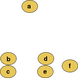
Figure 7.1: Raw data
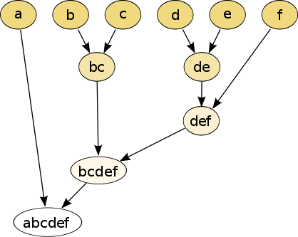
Figure 7.2: The hierarchical clustering dendrogram
With a top-down strategy, one instead starts with all observations in one cluster and then recursively split each cluster to form a hierarchy. One of the advantages of this strategy is that the method is deterministic.
7.1.3.2 k-means
In k-means clustering, the goal is to partition N objects (cells) into k different clusters. In an iterative manner, cluster centers are assigned and each cell is assigned to its nearest cluster:
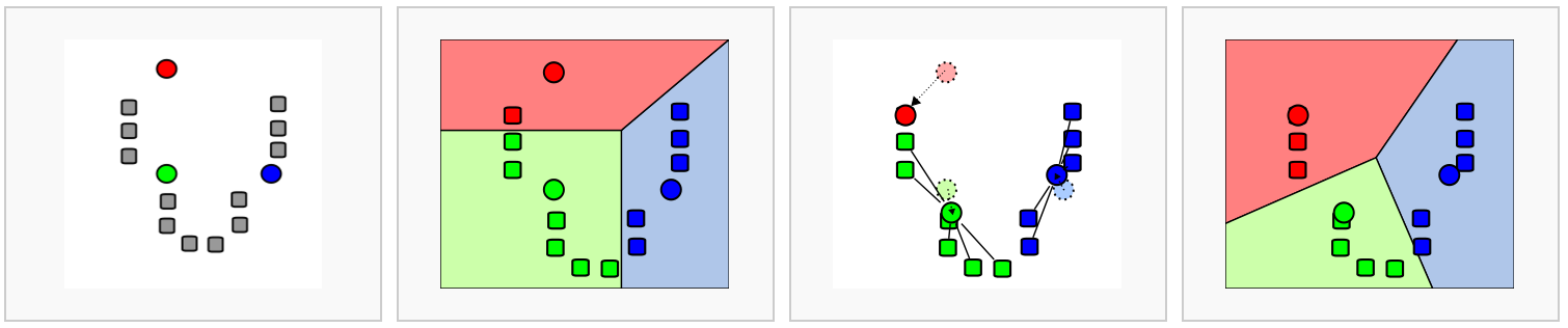
Figure 7.3: Schematic representation of the k-means clustering
Most methods for scRNA-seq analysis includes a k-means step at some point.
7.1.3.3 Graph-based methods
Over the last two decades there has been a lot of interest in analyzing networks in various domains. One goal is to identify group or modules of nodes in a network.
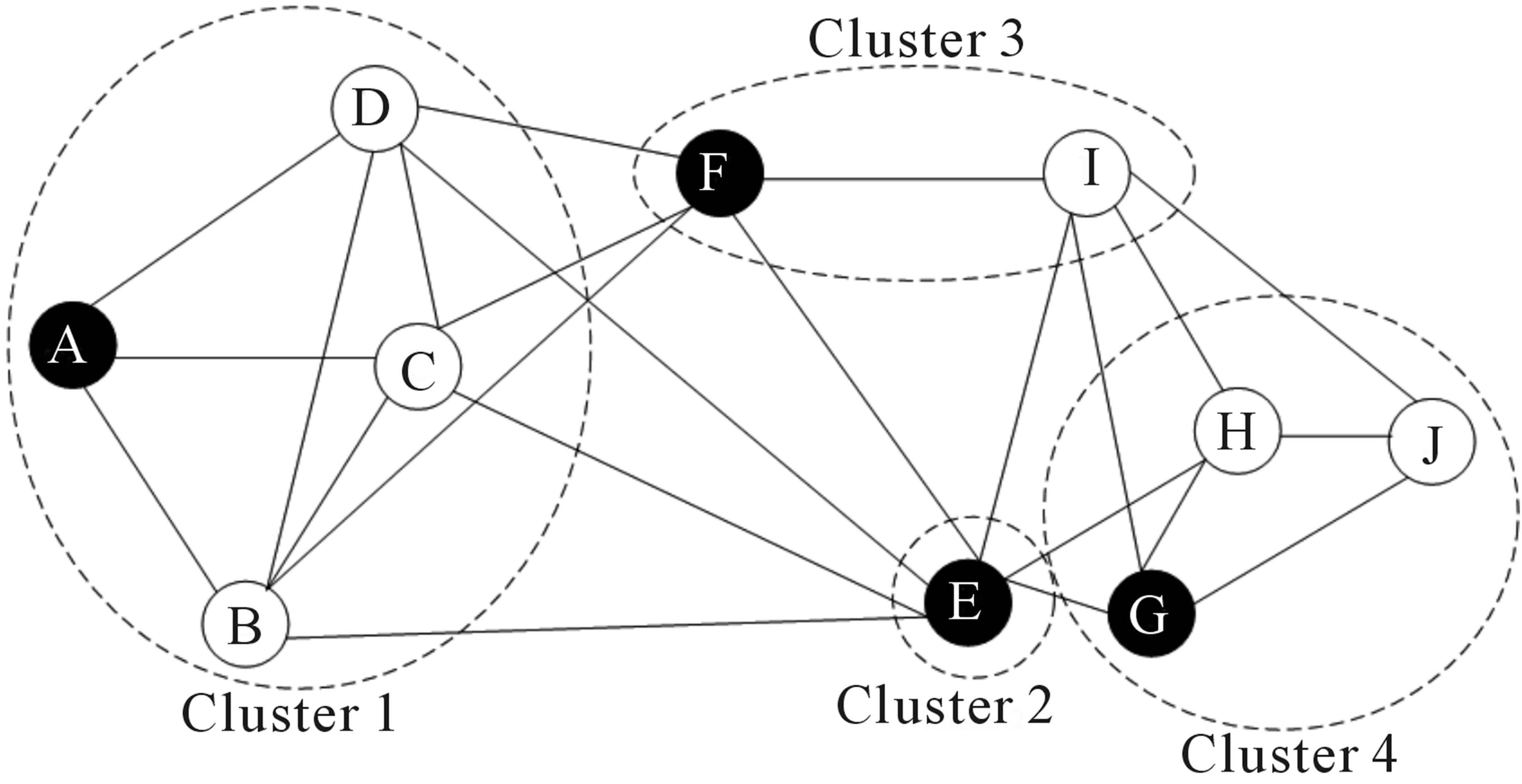
Figure 7.4: Schematic representation of the graph network
Some of these methods can be applied to scRNA-seq data by building a graph where each node represents a cell. Note that constructing the graph and assigning weights to the edges is not trivial. One advantage of graph-based methods is that some of them are very computationally efficient and can be applied to networks containing millions of nodes.
7.1.4 Challenges in clustering
- What is the number of clusters k?
- What is a cell type?
- Scalability: in the last few years the number of cells in scRNA-seq experiments has grown by several orders of magnitude from ~\(10^2\) to ~\(10^6\)
- Tools can be not user-friendly
7.1.5 Tools for scRNA-seq data
7.1.5.1 SINCERA
- SINCERA (Guo et al. 2015) is based on hierarchical clustering
- Data is converted to z-scores before clustering
- Identify k by finding the first singleton cluster in the hierarchy
7.1.5.2 SC3
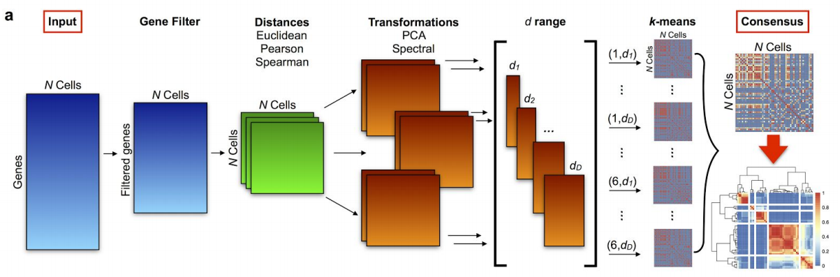
Figure 7.5: SC3 pipeline
- SC3 (Kiselev et al. 2017) is based on PCA and spectral dimensionality reductions
- Utilises k-means
- Additionally performs the consensus clustering
7.1.5.4 Seurat clustering
Seurat clustering is based on a community detection approach similar to SNN-Cliq and to one previously proposed for analyzing CyTOF data (Levine et al. 2015). Since Seurat has become more like an all-in-one tool for scRNA-seq data analysis we dedicate a separate chapter to discuss it in more details (see below).
7.1.6 Comparing clustering
To compare two sets of clustering labels we can use adjusted Rand index. The index is a measure of the similarity between two data clusterings. Values of the adjusted Rand index lie in \([0;1]\) interval, where \(1\) means that two clusterings are identical and \(0\) means the level of similarity expected by chance.
7.2 Clustering example
library(pcaMethods)
library(SC3)
library(scater)
library(SingleCellExperiment)
library(pheatmap)
library(mclust)
set.seed(1234567)
To illustrate clustering of scRNA-seq data, we consider the Deng dataset of cells from developing mouse embryo (Deng et al. 2014). We have preprocessed the dataset and created a SingleCellExperiment object in advance. We have also annotated the cells with the cell types identified in the original publication (it is the cell_type2 column in the colData slot).
7.2.1 Deng dataset
Let’s load the data and look at it:
deng <- readRDS("data/deng/deng-reads.rds")Let’s look at the cell type annotation:
table(colData(deng)$cell_type2)##
## 16cell 4cell 8cell early2cell earlyblast late2cell lateblast
## 50 14 37 8 43 10 30
## mid2cell midblast zy
## 12 60 4A simple PCA analysis already separates some strong cell types and provides some insights in the data structure:
deng <- runPCA(deng)
plotPCA(deng, colour_by = "cell_type2")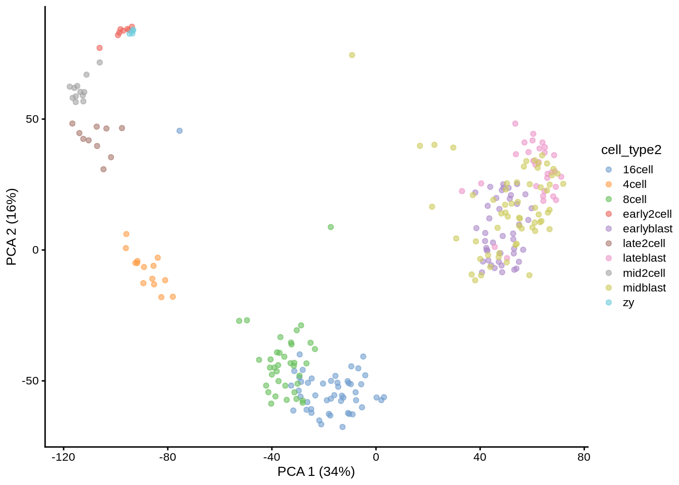
As you can see, the early cell types separate quite well, but the three blastocyst timepoints are more difficult to distinguish.
7.2.2 SC3
Let’s run SC3 clustering on the Deng data. The advantage of the SC3 is that it can directly ingest a SingleCellExperiment object.
Now let’s image we do not know the number of clusters k (cell types). SC3 can estimate a number of clusters for you:
deng <- sc3_estimate_k(deng)## Estimating k...metadata(deng)$sc3$k_estimation## [1] 6Interestingly, the number of cell types predicted by SC3 is smaller than in the original data annotation. However, if early, mid and late stages of different cell types are combined together, we will have exactly 6 cell types. We store the merged cell types in cell_type1 column of the colData slot:
plotPCA(deng, colour_by = "cell_type1")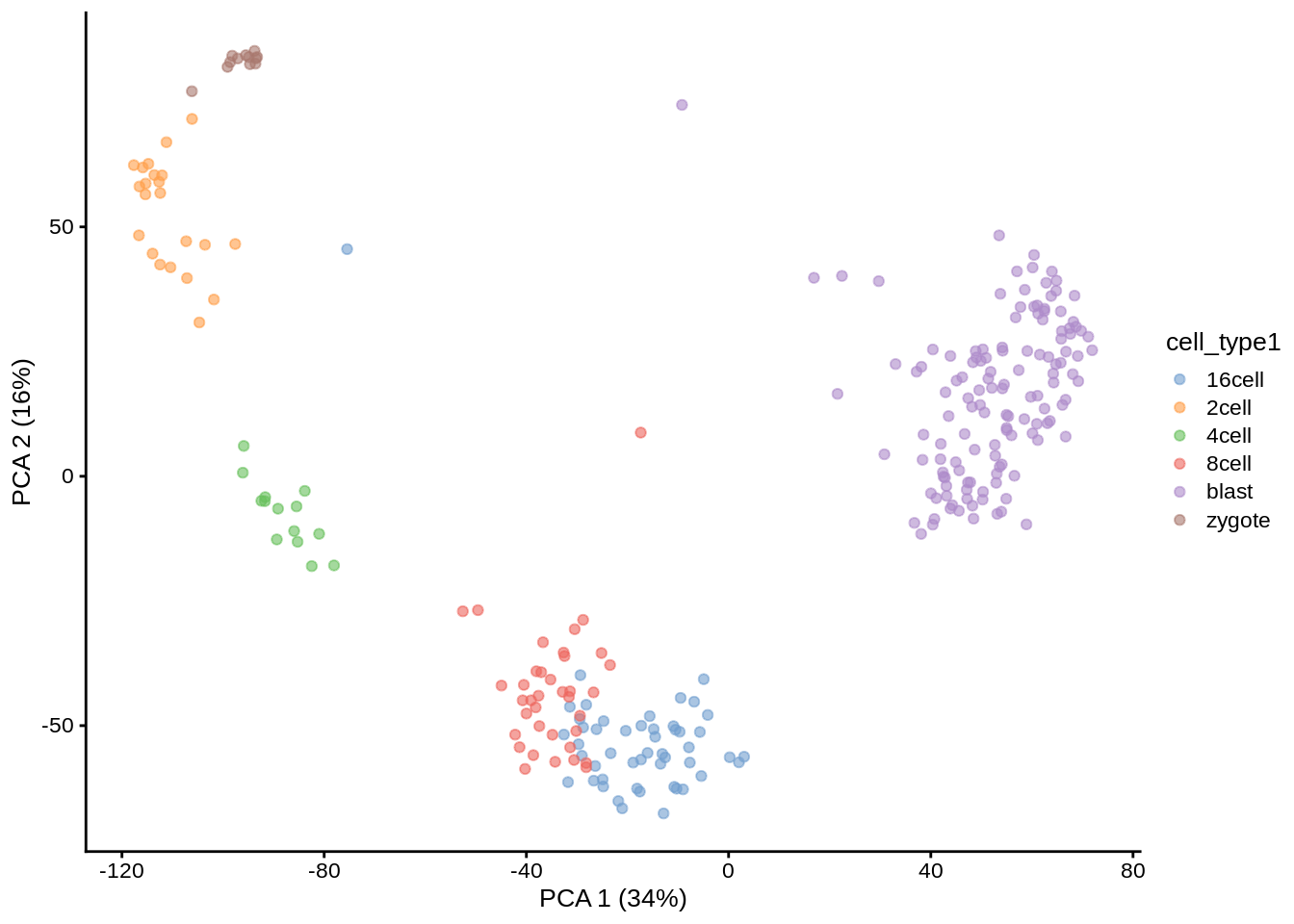
Now we are ready to run SC3 (we also ask it to calculate biological properties of the clusters):
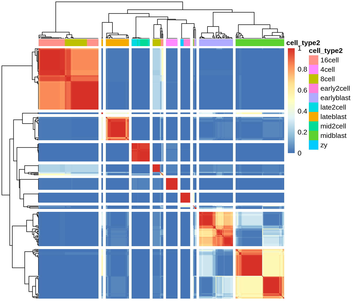
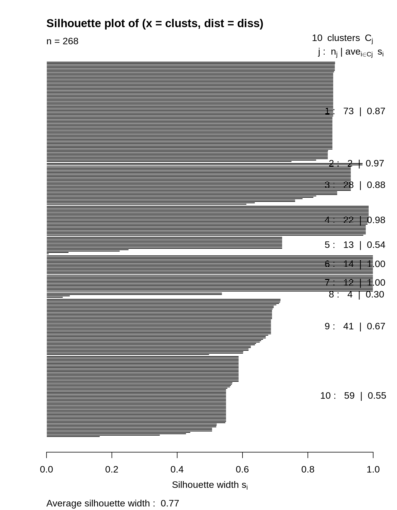
deng <- sc3(deng, ks = 10, biology = TRUE, n_cores = 1)## Setting SC3 parameters...## Calculating distances between the cells...## Performing transformations and calculating eigenvectors...## Performing k-means clustering...## Calculating consensus matrix...## Calculating biology...SC3 result consists of several different outputs (please look in (Kiselev et al. 2017) and SC3 vignette for more details). Here we show some of them:
Consensus matrix:
Silhouette plot:
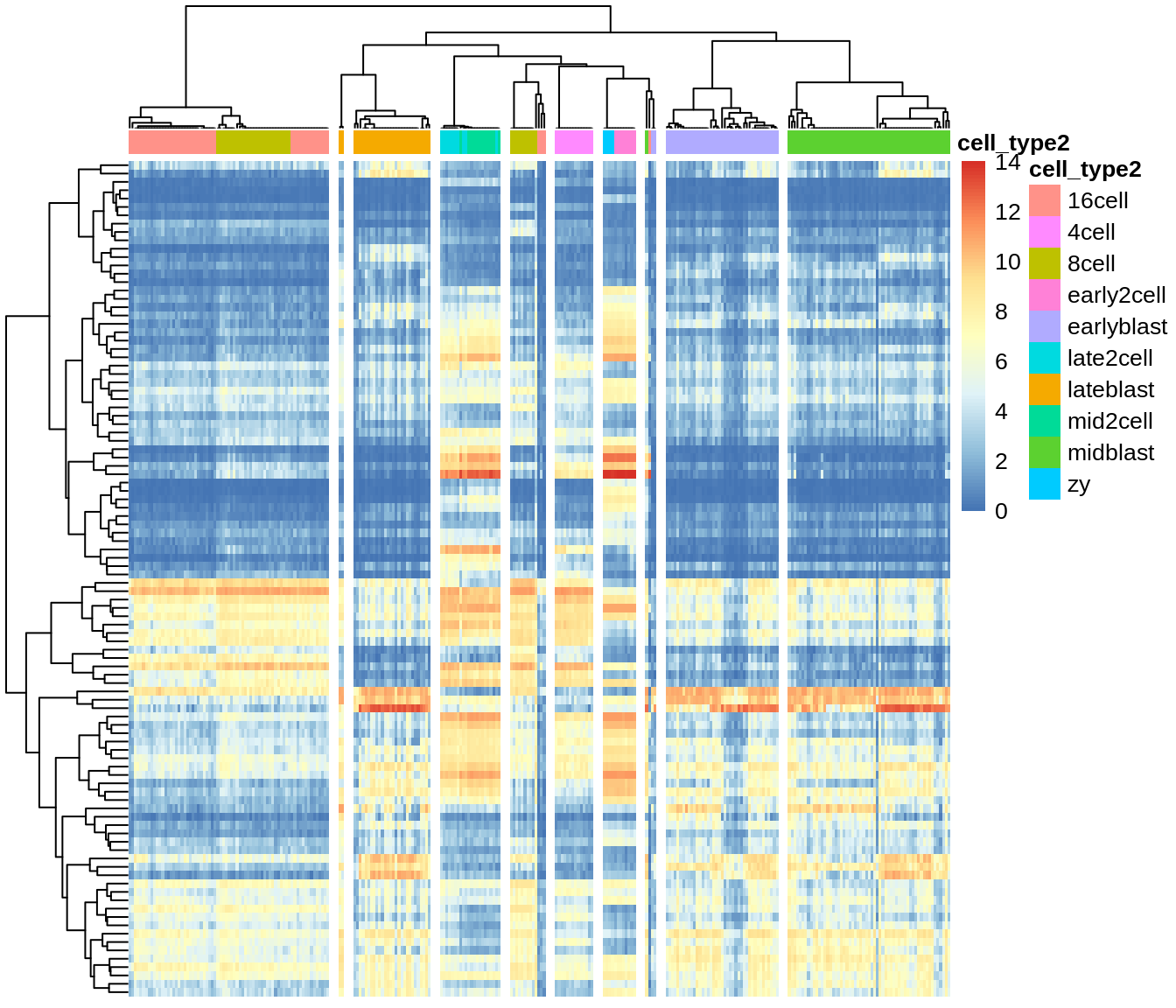
Heatmap of the expression matrix:
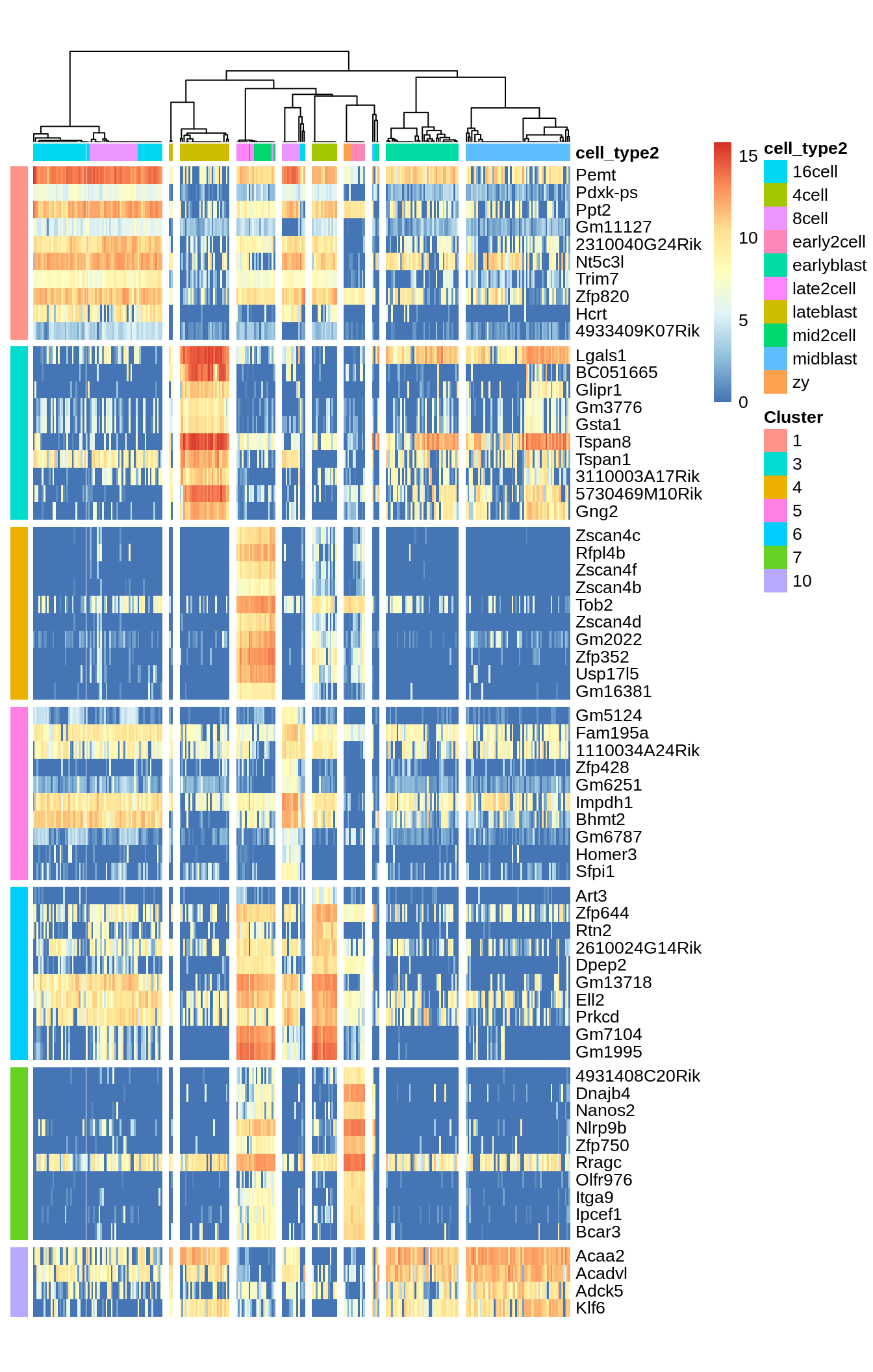
Identified marker genes:
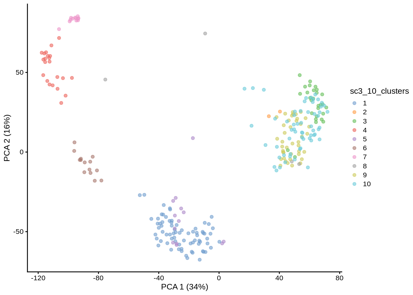
PCA plot with highlighted SC3 clusters:
Compare the results of SC3 clustering with the original publication cell type labels:
## [1] 0.7804189Note SC3 can also be run in an interactive Shiny session:
This command will open SC3 in a web browser.
Note Due to direct calculation of distances SC3 becomes very slow when the number of cells is \(>5000\). For large datasets containing up to \(10^5\) cells we recomment using Seurat (see chapter ??).
Exercise 1: Run
SC3for \(k\) from 8 to 12 and explore different clustering solutions in your web browser.Exercise 2: Which clusters are the most stable when \(k\) is changed from 8 to 12? (Look at the “Stability” tab)
Exercise 3: Check out differentially expressed genes and marker genes for the obtained clusterings. Please use \(k=10\).
Exercise 4: Change the marker genes threshold (the default is 0.85). Does SC3 find more marker genes?
7.2.3 tSNE + kmeans
tSNE plots that we saw before (??) when used the scater package are made by using the Rtsne and ggplot2 packages. Here we will do the same: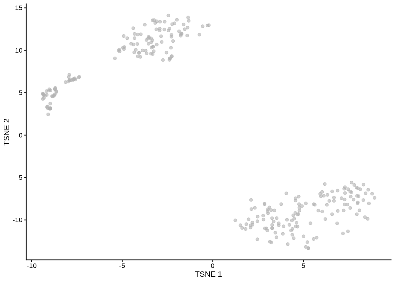
Figure 7.6: tSNE map of the patient data
Note that all points on the plot above are black. This is different from what we saw before, when the cells were coloured based on the annotation. Here we do not have any annotation and all cells come from the same batch, therefore all dots are black.
Now we are going to apply k-means clustering algorithm to the cloud of points on the tSNE map. How many groups do you see in the cloud?
We will start with \(k=8\):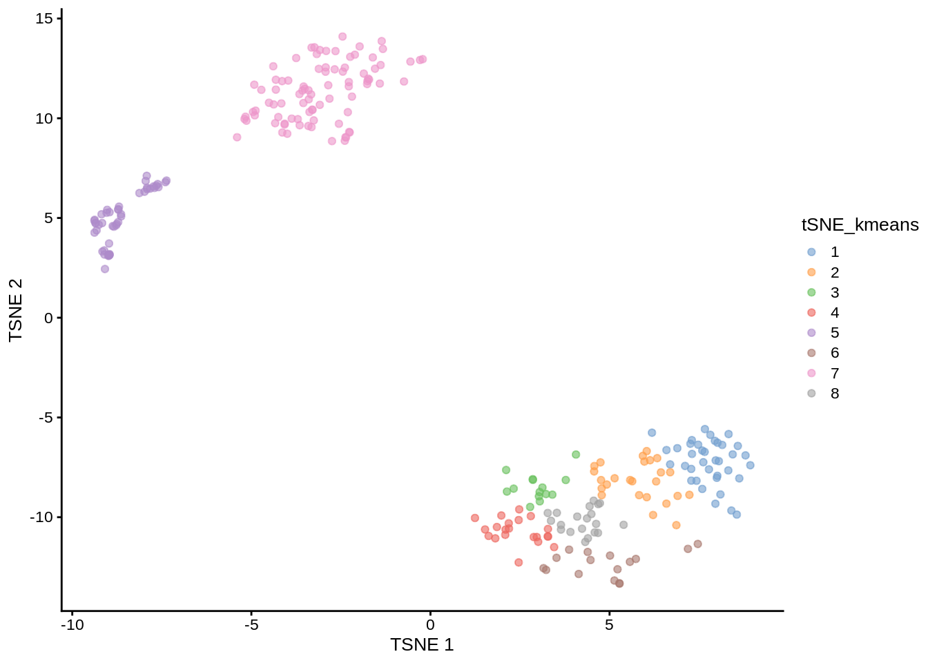
Figure 7.7: tSNE map of the patient data with 8 colored clusters, identified by the k-means clustering algorithm
Exercise 7: Make the same plot for \(k=10\).
Exercise 8: Compare the results between tSNE+kmeans and the original publication cell types. Can the results be improved by changing the perplexity parameter?
Our solution:
## [1] 0.4972803As you may have noticed, tSNE+kmeans is stochastic and gives different results every time they are run. To get a better overview of the solutions, we need to run the methods multiple times. SC3 is also stochastic, but thanks to the consensus step, it is more robust and less likely to produce different outcomes.
7.2.4 SINCERA
As mentioned in the previous chapter SINCERA is based on hierarchical clustering. One important thing to keep in mind is that it performs a gene-level z-score transformation before doing clustering:
# perform gene-by-gene per-sample z-score transformation
dat <- apply(input, 1, function(y) scRNA.seq.funcs::z.transform.helper(y))
# hierarchical clustering
dd <- as.dist((1 - cor(t(dat), method = "pearson"))/2)
hc <- hclust(dd, method = "average")
If the number of cluster is not known SINCERA can identify k as the minimum height of the hierarchical tree that generates no more than a specified number of singleton clusters (clusters containing only 1 cell):
num.singleton <- 0
kk <- 1
for (i in 2:dim(dat)[2]) {
    clusters <- cutree(hc, k = i)
    clustersizes <- as.data.frame(table(clusters))
    singleton.clusters <- which(clustersizes$Freq < 2)
    if (length(singleton.clusters) <= num.singleton) {
        kk <- i
    } else {
        break;
    }
}
cat(kk)
## 6Let’s now visualize the SINCERA results as a heatmap:
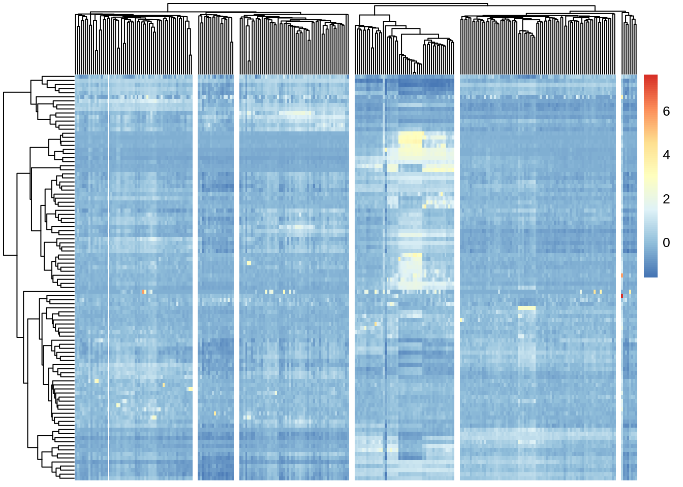
Figure 7.8: Clustering solutions of SINCERA method using found \(k\)
Exercise 10: Compare the results between SINCERA and the original publication cell types.
Our solution:
## [1] 0.3823537Exercise 11: Is using the singleton cluster criteria for finding k a good idea?
7.2.5 sessionInfo()
View session info
## R version 4.2.1 (2022-06-23)
## Platform: x86_64-pc-linux-gnu (64-bit)
## Running under: Ubuntu 20.04.2 LTS
##
## Matrix products: default
## BLAS:   /usr/lib/x86_64-linux-gnu/blas/libblas.so.3.9.0
## LAPACK: /usr/lib/x86_64-linux-gnu/lapack/liblapack.so.3.9.0
##
## locale:
##  [1] LC_CTYPE=en_US.UTF-8       LC_NUMERIC=C
##  [3] LC_TIME=en_US.UTF-8        LC_COLLATE=en_US.UTF-8
##  [5] LC_MONETARY=en_US.UTF-8    LC_MESSAGES=en_US.UTF-8
##  [7] LC_PAPER=en_US.UTF-8       LC_NAME=C
##  [9] LC_ADDRESS=C               LC_TELEPHONE=C
## [11] LC_MEASUREMENT=en_US.UTF-8 LC_IDENTIFICATION=C
##
## attached base packages:
## [1] stats4    stats     graphics  grDevices utils     datasets  methods
## [8] base
##
## other attached packages:
##  [1] mclust_5.4.10               pheatmap_1.0.12
##  [3] scater_1.24.0               ggplot2_3.3.6
##  [5] scuttle_1.6.2               SingleCellExperiment_1.18.0
##  [7] SummarizedExperiment_1.26.1 GenomicRanges_1.48.0
##  [9] GenomeInfoDb_1.32.2         IRanges_2.30.0
## [11] S4Vectors_0.34.0            MatrixGenerics_1.8.1
## [13] matrixStats_0.62.0          SC3_1.24.0
## [15] pcaMethods_1.88.0           Biobase_2.56.0
## [17] BiocGenerics_0.42.0         knitr_1.39
##
## loaded via a namespace (and not attached):
##   [1] Rtsne_0.16                ggbeeswarm_0.6.0
##   [3] colorspace_2.0-3          ellipsis_0.3.2
##   [5] class_7.3-20              XVector_0.36.0
##   [7] BiocNeighbors_1.14.0      proxy_0.4-27
##   [9] farver_2.1.1              ggrepel_0.9.1
##  [11] fansi_1.0.3               mvtnorm_1.1-3
##  [13] scRNA.seq.funcs_0.1.0     codetools_0.2-18
##  [15] sparseMatrixStats_1.8.0   doParallel_1.0.17
##  [17] robustbase_0.95-0         polynom_1.4-1
##  [19] jsonlite_1.8.0            cluster_2.1.3
##  [21] shiny_1.7.1               rrcov_1.7-0
##  [23] compiler_4.2.1            assertthat_0.2.1
##  [25] Matrix_1.4-1              fastmap_1.1.0
##  [27] cli_3.3.0                 later_1.3.0
##  [29] BiocSingular_1.12.0       htmltools_0.5.2
##  [31] tools_4.2.1               rsvd_1.0.5
##  [33] gtable_0.3.0              glue_1.6.2
##  [35] GenomeInfoDbData_1.2.8    dplyr_1.0.9
##  [37] doRNG_1.8.2               Rcpp_1.0.9
##  [39] jquerylib_0.1.4           vctrs_0.4.1
##  [41] iterators_1.0.14          DelayedMatrixStats_1.18.0
##  [43] xfun_0.31                 stringr_1.4.0
##  [45] beachmat_2.12.0           mime_0.12
##  [47] lifecycle_1.0.1           irlba_2.3.5
##  [49] hypergeo_1.2-13           rngtools_1.5.2
##  [51] WriteXLS_6.4.0            statmod_1.4.36
##  [53] DEoptimR_1.0-11           MASS_7.3-58
##  [55] zlibbioc_1.42.0           scales_1.2.0
##  [57] promises_1.2.0.1          parallel_4.2.1
##  [59] RColorBrewer_1.1-3        yaml_2.3.5
##  [61] gridExtra_2.3             sass_0.4.1
##  [63] stringi_1.7.8             highr_0.9
##  [65] pcaPP_2.0-2               foreach_1.5.2
##  [67] ScaledMatrix_1.4.0        orthopolynom_1.0-6
##  [69] e1071_1.7-11              contfrac_1.1-12
##  [71] BiocParallel_1.30.3       moments_0.14.1
##  [73] rlang_1.0.4               pkgconfig_2.0.3
##  [75] bitops_1.0-7              evaluate_0.15
##  [77] lattice_0.20-45           ROCR_1.0-11
##  [79] purrr_0.3.4               labeling_0.4.2
##  [81] cowplot_1.1.1             tidyselect_1.1.2
##  [83] deSolve_1.32              magrittr_2.0.3
##  [85] bookdown_0.27             R6_2.5.1
##  [87] generics_0.1.3            DelayedArray_0.22.0
##  [89] DBI_1.1.3                 pillar_1.7.0
##  [91] withr_2.5.0               RCurl_1.98-1.7
##  [93] tibble_3.1.7              crayon_1.5.1
##  [95] utf8_1.2.2                rmarkdown_2.14
##  [97] viridis_0.6.2             grid_4.2.1
##  [99] digest_0.6.29             xtable_1.8-4
## [101] httpuv_1.6.5              elliptic_1.4-0
## [103] munsell_0.5.0             beeswarm_0.4.0
## [105] viridisLite_0.4.0         vipor_0.4.5
## [107] bslib_0.3.1
7.3 Differential Expression (DE) Analysis
7.3.1 Bulk RNA-seq
One of the most common types of analyses when working with bulk RNA-seq data is to identify differentially expressed genes. By comparing the genes that change between two conditions, e.g. mutant and wild-type or stimulated and unstimulated, it is possible to characterize the molecular mechanisms underlying the change.
Several different methods, e.g. DESeq2 and edgeR, have been developed for bulk RNA-seq. Moreover, there are also extensive datasets available where the RNA-seq data has been validated using RT-qPCR. These data can be used to benchmark DE finding algorithms and the available evidence suggests that the algorithms are performing quite well.
7.3.2 Single Cell RNA-seq
In contrast to bulk RNA-seq, in scRNA-seq we usually do not have a defined set of experimental conditions. Instead, as was shown in a previous chapter (7.2) we can identify the cell groups by using an unsupervised clustering approach. Once the groups have been identified one can find differentially expressed genes either by comparing the differences in variance between the groups (like the Kruskal-Wallis test implemented in SC3), or by comparing gene expression between clusters in a pairwise manner. In the following chapter we will mainly consider tools developed for pairwise comparisons.
7.3.3 Differences in Distribution
Unlike bulk RNA-seq, we generally have a large number of samples (i.e. cells) for each group we are comparing in single-cell experiments. Thus we can take advantage of the whole distribution of expression values in each group to identify differences between groups rather than only comparing estimates of mean-expression as is standard for bulk RNASeq.
There are two main approaches to comparing distributions. Firstly, we can use existing statistical models/distributions and fit the same type of model to the expression in each group then test for differences in the parameters for each model, or test whether the model fits better if a particular paramter is allowed to be different according to group. For instance in Chapter 6.6 we used edgeR to test whether allowing mean expression to be different in different batches significantly improved the fit of a negative binomial model of the data.
Alternatively, we can use a non-parametric test which does not assume that expression values follow any particular distribution, e.g. the Kolmogorov-Smirnov test (KS-test). Non-parametric tests generally convert observed expression values to ranks and test whether the distribution of ranks for one group are signficantly different from the distribution of ranks for the other group. However, some non-parametric methods fail in the presence of a large number of tied values, such as the case for dropouts (zeros) in single-cell RNA-seq expression data. Moreover, if the conditions for a parametric test hold, then it will typically be more powerful than a non-parametric test.
7.3.4 Models of single-cell RNA-seq data
The most common model of scRNA-seq data is the negative binomial model:
set.seed(1)
hist(
    rnbinom(
        1000,
        mu = 10,
        size = 100),
    col = "grey50",
    xlab = "Read Counts",
    main = "Negative Binomial"
)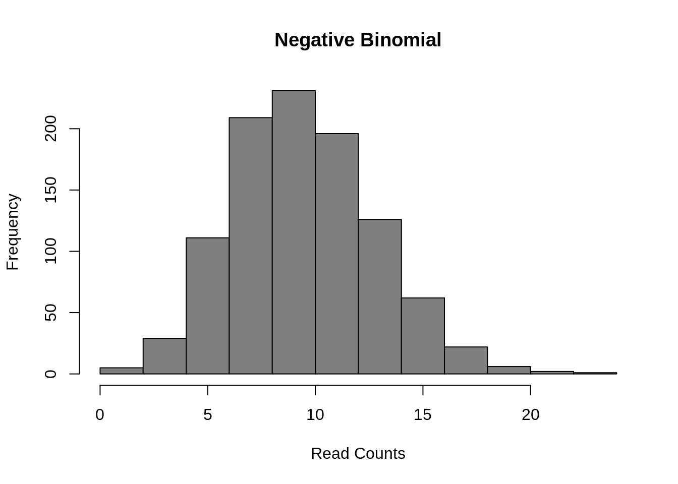
Figure 7.9: Negative Binomial distribution of read counts for a single gene across 1000 cells
Mean: \(\mu = mu\)
Variance: \(\sigma^2 = mu + mu^2/size\)
It is parameterized by the mean expression (mu) and the dispersion (size), which is inversely related to the variance. The negative binomial model fits bulk RNA-seq data very well and it is used for most statistical methods designed for such data. In addition, it has been show to fit the distribution of molecule counts obtained from data tagged by unique molecular identifiers (UMIs) quite well (Grun et al. 2014, Islam et al. 2011).
However, a raw negative binomial model does not fit full-length transcript data as well due to the high dropout rates relative to the non-zero read counts. For this type of data a variety of zero-inflated negative binomial models have been proposed (e.g. MAST, SCDE).
d <- 0.5;
counts <- rnbinom(
    1000,
    mu = 10,
    size = 100
)
counts[runif(1000) < d] <- 0
hist(
    counts,
    col = "grey50",
    xlab = "Read Counts",
    main = "Zero-inflated NB"
)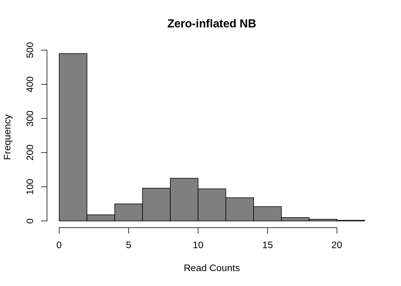
Figure 7.10: Zero-inflated Negative Binomial distribution
Mean: \(\mu = mu \cdot (1 - d)\)
Variance: \(\sigma^2 = \mu \cdot (1-d) \cdot (1 + d \cdot \mu + \mu / size)\)
These models introduce a new parameter \(d\), for the dropout rate, to the negative binomial model. As we saw in Chapter 19, the dropout rate of a gene is strongly correlated with the mean expression of the gene. Different zero-inflated negative binomial models use different relationships between mu and d and some may fit \(\mu\) and \(d\) to the expression of each gene independently.
Finally, several methods use a Poisson-Beta distribution which is based on a mechanistic model of transcriptional bursting. There is strong experimental support for this model (Kim and Marioni, 2013) and it provides a good fit to scRNA-seq data but it is less easy to use than the negative-binomial models and much less existing methods upon which to build than the negative binomial model.
a <- 0.1
b <- 0.1
g <- 100
lambdas <- rbeta(1000, a, b)
counts <- sapply(g*lambdas, function(l) {rpois(1, lambda = l)})
hist(
counts,
col = "grey50",
xlab = "Read Counts",
main = "Poisson-Beta"
)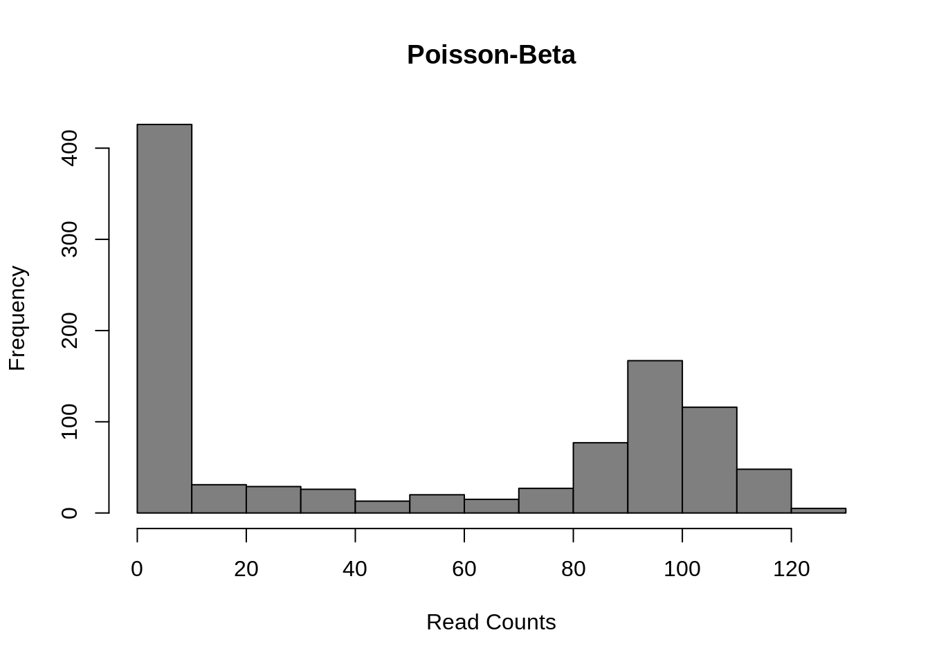 Mean:
\(\mu = g \cdot a / (a + b)\)
Mean:
\(\mu = g \cdot a / (a + b)\)
Variance: \(\sigma^2 = g^2 \cdot a \cdot b/((a + b + 1) \cdot (a + b)^2)\)
This model uses three parameters: \(a\) the rate of activation of transcription; \(b\) the rate of inhibition of transcription; and \(g\) the rate of transcript production while transcription is active at the locus. Differential expression methods may test each of the parameters for differences across groups or only one (often \(g\)).
All of these models may be further expanded to explicitly account for other sources of gene expression differences such as batch-effect or library depth depending on the particular DE algorithm.
Exercise: Vary the parameters of each distribution to explore how they affect the distribution of gene expression. How similar are the Poisson-Beta and Negative Binomial models?
7.4 DE in a Real Dataset
library(scRNA.seq.funcs)
library(edgeR)
#library(monocle)
library(MAST)
library(ROCR)
set.seed(1)
7.4.1 Introduction
To test different single-cell differential expression methods we will be using the Blischak dataset from Chapters 7-17. For this experiment bulk RNA-seq data for each cell-line was generated in addition to single-cell data. We will use the differentially expressed genes identified using standard methods on the respective bulk data as the ground truth for evaluating the accuracy of each single-cell method. To save time we have pre-computed these for you. You can run the commands below to load these data.
DE <- read.table("data/tung/TPs.txt")
notDE <- read.table("data/tung/TNs.txt")
GroundTruth <- list(
    DE = as.character(unlist(DE)),
    notDE = as.character(unlist(notDE))
)
This ground truth has been produce for the comparison of individual NA19101 to NA19239. Now load the respective single-cell data:
molecules <- read.table("data/tung/molecules.txt", sep = "\t")
anno <- read.table("data/tung/annotation.txt", sep = "\t", header = TRUE)
keep <- anno[,1] == "NA19101" | anno[,1] == "NA19239"
data <- molecules[,keep]
group <- anno[keep,1]
batch <- anno[keep,4]
# remove genes that aren't expressed in at least 6 cells
gkeep <- rowSums(data > 0) > 5;
counts <- data[gkeep,]
# Library size normalization
lib_size = colSums(counts)
norm <- t(t(counts)/lib_size * median(lib_size))
# Variant of CPM for datasets with library sizes of fewer than 1 mil molecules
Now we will compare various single-cell DE methods. Note that we will only be running methods which are available as R-packages and run relatively quickly.
7.4.2 Kolmogorov-Smirnov Test
The types of test that are easiest to work with are non-parametric ones. The most commonly used non-parametric test is the Kolmogorov-Smirnov test (KS-test) and we can use it to compare the distributions for each gene in the two individuals. The KS-test quantifies the distance between the empirical cummulative distributions of the expression of each gene in each of the two populations. It is sensitive to changes in mean experession and changes in variability. However it assumes data is continuous and may perform poorly when data contains a large number of identical values (eg. zeros). Another issue with the KS-test is that it can be very sensitive for large sample sizes and thus it may end up as significant even though the magnitude of the difference is very small.
)](figures/KS2_Example.png)
Figure 7.11: Illustration of the two-sample Kolmogorov–Smirnov statistic. Red and blue lines each correspond to an empirical distribution function, and the black arrow is the two-sample KS statistic. (taken from here)
Now run the test:
pVals <- apply(
    norm, 1, function(x) {
        ks.test(
            x[group == "NA19101"],
            x[group == "NA19239"]
        )$p.value
    }
)
# multiple testing correction
pVals <- p.adjust(pVals, method = "fdr")
This code “applies” the function to each row (specified by 1) of the expression matrix, data. In the function we are returning just the p.value from the ks.test output. We can now consider how many of the ground truth positive and negative DE genes are detected by the KS-test:
7.4.2.1 Evaluating Accuracy
sigDE <- names(pVals)[pVals < 0.05]
length(sigDE)
## [1] 5095# Number of KS-DE genes
sum(GroundTruth$DE %in% sigDE) ## [1] 792# Number of KS-DE genes that are true DE genes
sum(GroundTruth$notDE %in% sigDE)## [1] 3190# Number of KS-DE genes that are truly not-DEAs you can see many more of our ground truth negative genes were identified as DE by the KS-test (false positives) than ground truth positive genes (true positives), however this may be due to the larger number of notDE genes thus we typically normalize these counts as the True positive rate (TPR), TP/(TP + FN), and False positive rate (FPR), FP/(FP+TP).
tp <- sum(GroundTruth$DE %in% sigDE)
fp <- sum(GroundTruth$notDE %in% sigDE)
tn <- sum(GroundTruth$notDE %in% names(pVals)[pVals >= 0.05])
fn <- sum(GroundTruth$DE %in% names(pVals)[pVals >= 0.05])
tpr <- tp/(tp + fn)
fpr <- fp/(fp + tn)
cat(c(tpr, fpr))
## 0.7346939 0.2944706Now we can see the TPR is much higher than the FPR indicating the KS test is identifying DE genes.
So far we’ve only evaluated the performance at a single significance threshold. Often it is informative to vary the threshold and evaluate performance across a range of values. This is then plotted as a receiver-operating-characteristic curve (ROC) and a general accuracy statistic can be calculated as the area under this curve (AUC). We will use the ROCR package to facilitate this plotting.
# Only consider genes for which we know the ground truth
pVals <- pVals[names(pVals) %in% GroundTruth$DE |
               names(pVals) %in% GroundTruth$notDE]
truth <- rep(1, times = length(pVals));
truth[names(pVals) %in% GroundTruth$DE] = 0;
pred <- ROCR::prediction(pVals, truth)
perf <- ROCR::performance(pred, "tpr", "fpr")
ROCR::plot(perf)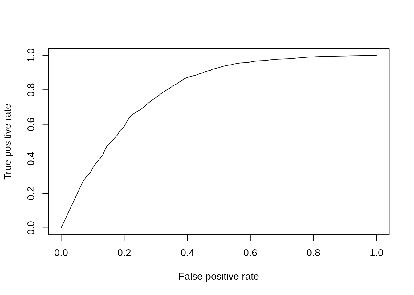
Figure 7.12: ROC curve for KS-test.
aucObj <- ROCR::performance(pred, "auc")
aucObj@y.values[[1]] # AUC
## [1] 0.7954796Finally to facilitate the comparisons of other DE methods let’s put this code into a function so we don’t need to repeat it:
DE_Quality_AUC <- function(pVals) {
    pVals <- pVals[names(pVals) %in% GroundTruth$DE |
                   names(pVals) %in% GroundTruth$notDE]
    truth <- rep(1, times = length(pVals));
    truth[names(pVals) %in% GroundTruth$DE] = 0;
    pred <- ROCR::prediction(pVals, truth)
    perf <- ROCR::performance(pred, "tpr", "fpr")
    ROCR::plot(perf)
    aucObj <- ROCR::performance(pred, "auc")
    return(aucObj@y.values[[1]])
}
7.4.3 Wilcox/Mann-Whitney-U Test
The Wilcox-rank-sum test is another non-parametric test, but tests specifically if values in one group are greater/less than the values in the other group. Thus it is often considered a test for difference in median expression between two groups; whereas the KS-test is sensitive to any change in distribution of expression values.
pVals <- apply(
    norm, 1, function(x) {
        wilcox.test(
            x[group == "NA19101"],
            x[group == "NA19239"]
        )$p.value
    }
)
# multiple testing correction
pVals <- p.adjust(pVals, method = "fdr")
DE_Quality_AUC(pVals)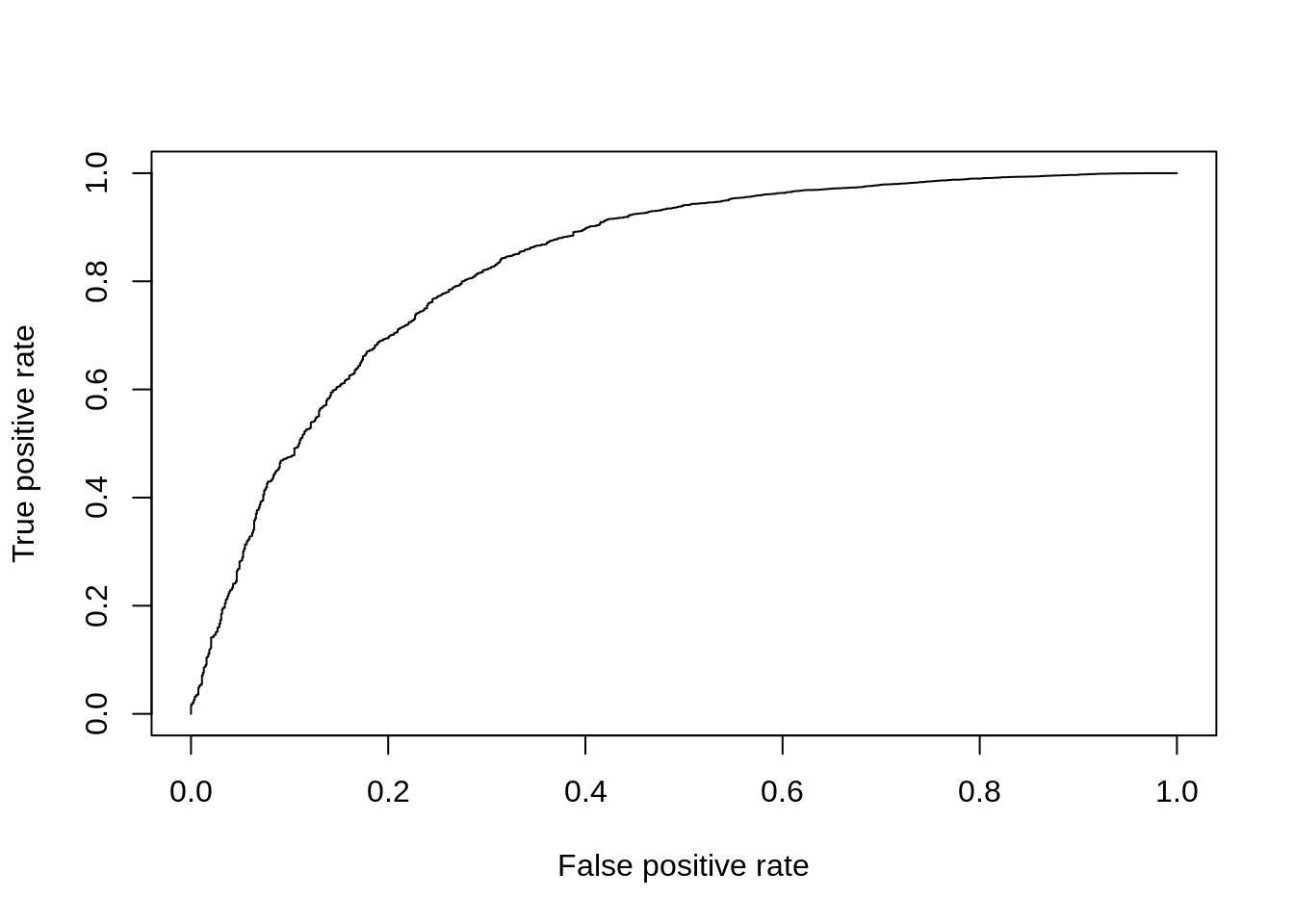
Figure 7.13: ROC curve for Wilcox test.
## [1] 0.83203267.4.4 edgeR
We’ve already used edgeR for differential expression in Chapter 6.6. edgeR is based on a negative binomial model of gene expression and uses a generalized linear model (GLM) framework, the enables us to include other factors such as batch to the model.
dge <- DGEList(
    counts = counts,
    norm.factors = rep(1, length(counts[1,])),
    group = group
)
group_edgeR <- factor(group)
design <- model.matrix(~ group_edgeR)
dge <- estimateDisp(dge, design = design, trend.method = "none")
fit <- glmFit(dge, design)
res <- glmLRT(fit)
pVals <- res$table[,4]
names(pVals) <- rownames(res$table)

pVals <- p.adjust(pVals, method = "fdr")
DE_Quality_AUC(pVals)
Figure 7.14: ROC curve for edgeR.
## [1] 0.84667647.4.5 MAST
MAST is based on a zero-inflated negative binomial model. It tests for differential expression using a hurdle model to combine tests of discrete (0 vs not zero) and continuous (non-zero values) aspects of gene expression. Again this uses a linear modelling framework to enable complex models to be considered.
log_counts <- log(counts + 1) / log(2)
fData <- data.frame(names = rownames(log_counts))
rownames(fData) <- rownames(log_counts);
cData <- data.frame(cond = group)
rownames(cData) <- colnames(log_counts)

obj <- FromMatrix(as.matrix(log_counts), cData, fData)
colData(obj)$cngeneson <- scale(colSums(assay(obj) > 0))
cond <- factor(colData(obj)$cond)

# Model expression as function of condition & number of detected genes
zlmCond <- zlm(~ cond + cngeneson, obj)

summaryCond <- summary(zlmCond, doLRT = "condNA19239")
summaryDt <- summaryCond$datatable

summaryDt <- as.data.frame(summaryDt)
pVals <- unlist(summaryDt[summaryDt$component == "H",4]) # H = hurdle model
names(pVals) <- unlist(summaryDt[summaryDt$component == "H",1])
pVals <- p.adjust(pVals, method = "fdr")
DE_Quality_AUC(pVals)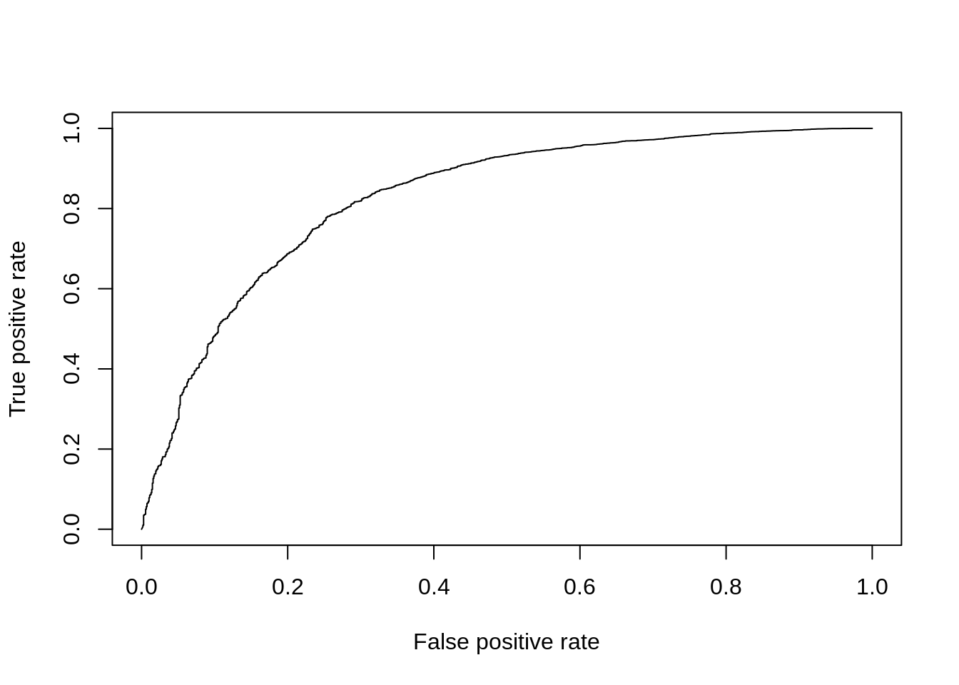
Figure 7.15: ROC curve for MAST.
## [1] 0.82840467.4.6 Slow Methods (>1h to run)
These methods are too slow to run today but we encourage you to try them out on your own:
7.4.7 BPSC
BPSC uses the Poisson-Beta model of single-cell gene expression, which we discussed in the previous chapter, and combines it with generalized linear models which we’ve already encountered when using edgeR. BPSC performs comparisons of one or more groups to a reference group (“control”) and can include other factors such as batches in the model.
library(BPSC)
bpsc_data <- norm[,batch=="NA19101.r1" | batch=="NA19239.r1"]
bpsc_group = group[batch=="NA19101.r1" | batch=="NA19239.r1"]

control_cells <- which(bpsc_group == "NA19101")
design <- model.matrix(~bpsc_group)
coef=2 # group label
res=BPglm(data=bpsc_data, controlIds=control_cells, design=design, coef=coef,
                estIntPar=FALSE, useParallel = FALSE)
pVals = res$PVAL
pVals <- p.adjust(pVals, method = "fdr")
DE_Quality_AUC(pVals)
7.4.8 SCDE
SCDE is the first single-cell specific DE method. It fits a zero-inflated negative binomial model to expression data using Bayesian statistics. The usage below tests for differences in mean expression of individual genes across groups but recent versions include methods to test for differences in mean expression or dispersion of groups of genes, usually representing a pathway.
library(scde)
cnts <- apply(
    counts,
    2,
    function(x) {
        storage.mode(x) <- 'integer'
        return(x)
    }
)
names(group) <- 1:length(group)
colnames(cnts) <- 1:length(group)
o.ifm <- scde::scde.error.models(
    counts = cnts,
    groups = group,
    n.cores = 1,
    threshold.segmentation = TRUE,
    save.crossfit.plots = FALSE,
    save.model.plots = FALSE,
    verbose = 0,
    min.size.entries = 2
)
priors <- scde::scde.expression.prior(
    models = o.ifm,
    counts = cnts,
    length.out = 400,
    show.plot = FALSE
)
resSCDE <- scde::scde.expression.difference(
    o.ifm,
    cnts,
    priors,
    groups = group,
    n.randomizations = 100,
    n.cores = 1,
    verbose = 0
)
# Convert Z-scores into 2-tailed p-values
pVals <- pnorm(abs(resSCDE$cZ), lower.tail = FALSE) * 2
DE_Quality_AUC(pVals)
7.4.9 sessionInfo()
View session info
## R version 4.2.1 (2022-06-23)
## Platform: x86_64-pc-linux-gnu (64-bit)
## Running under: Ubuntu 20.04.2 LTS
##
## Matrix products: default
## BLAS:   /usr/lib/x86_64-linux-gnu/blas/libblas.so.3.9.0
## LAPACK: /usr/lib/x86_64-linux-gnu/lapack/liblapack.so.3.9.0
##
## locale:
##  [1] LC_CTYPE=en_US.UTF-8       LC_NUMERIC=C
##  [3] LC_TIME=en_US.UTF-8        LC_COLLATE=en_US.UTF-8
##  [5] LC_MONETARY=en_US.UTF-8    LC_MESSAGES=en_US.UTF-8
##  [7] LC_PAPER=en_US.UTF-8       LC_NAME=C
##  [9] LC_ADDRESS=C               LC_TELEPHONE=C
## [11] LC_MEASUREMENT=en_US.UTF-8 LC_IDENTIFICATION=C
##
## attached base packages:
## [1] stats4    stats     graphics  grDevices utils     datasets  methods
## [8] base
##
## other attached packages:
##  [1] ROCR_1.0-11                 MAST_1.22.0
##  [3] SingleCellExperiment_1.18.0 SummarizedExperiment_1.26.1
##  [5] Biobase_2.56.0              GenomicRanges_1.48.0
##  [7] GenomeInfoDb_1.32.2         IRanges_2.30.0
##  [9] S4Vectors_0.34.0            BiocGenerics_0.42.0
## [11] MatrixGenerics_1.8.1        matrixStats_0.62.0
## [13] edgeR_3.38.1                limma_3.52.2
## [15] scRNA.seq.funcs_0.1.0       knitr_1.39
##
## loaded via a namespace (and not attached):
##  [1] sass_0.4.1             jsonlite_1.8.0         elliptic_1.4-0
##  [4] bslib_0.3.1            moments_0.14.1         assertthat_0.2.1
##  [7] statmod_1.4.36         highr_0.9              GenomeInfoDbData_1.2.8
## [10] progress_1.2.2         yaml_2.3.5             pillar_1.7.0
## [13] lattice_0.20-45        glue_1.6.2             digest_0.6.29
## [16] XVector_0.36.0         colorspace_2.0-3       htmltools_0.5.2
## [19] Matrix_1.4-1           plyr_1.8.7             pkgconfig_2.0.3
## [22] bookdown_0.27          zlibbioc_1.42.0        purrr_0.3.4
## [25] scales_1.2.0           Rtsne_0.16             tibble_3.1.7
## [28] generics_0.1.3         ggplot2_3.3.6          ellipsis_0.3.2
## [31] cli_3.3.0              magrittr_2.0.3         crayon_1.5.1
## [34] evaluate_0.15          fansi_1.0.3            MASS_7.3-58
## [37] prettyunits_1.1.1      tools_4.2.1            data.table_1.14.2
## [40] hms_1.1.1              lifecycle_1.0.1        stringr_1.4.0
## [43] munsell_0.5.0          locfit_1.5-9.6         DelayedArray_0.22.0
## [46] orthopolynom_1.0-6     compiler_4.2.1         jquerylib_0.1.4
## [49] contfrac_1.1-12        rlang_1.0.4            grid_4.2.1
## [52] RCurl_1.98-1.7         bitops_1.0-7           rmarkdown_2.14
## [55] hypergeo_1.2-13        gtable_0.3.0           codetools_0.2-18
## [58] abind_1.4-5            deSolve_1.32           DBI_1.1.3
## [61] reshape2_1.4.4         polynom_1.4-1          R6_2.5.1
## [64] dplyr_1.0.9            fastmap_1.1.0          utf8_1.2.2
## [67] stringi_1.7.8          Rcpp_1.0.9             vctrs_0.4.1
## [70] tidyselect_1.1.2       xfun_0.31