3 Processing Raw scRNA-Seq Sequencing Data: From Reads to a Count Matrix
3.1 Reference Genome and its Annotation
Most scRNA-seq experiments are done using human or mouse tissues, organoids, or cell cultures. Even though first drafts of these genomes were published about 20 years ago, assembly and annotation updates happen fairly regularly. There are two popular sources of assembly files: UCSC (their assemblies are named hg19, hg38, mm10, etc), and GRC (GRCh37, GRCh38, GRCm38). Major releases of UCSC and GRC assemblies are matched in main chromosomes (e.g. chr1 from hg38 = chr1 from GRCh38), but differ in additional contigs and so-called ALT loci, which change between minor releases (e.g. GRCh38.p13). More information can be obtained here and here. Genome assembly is usually distributed as a fasta file - a simple text file that includes sequence names and sequences.
Genome annotation process includes defining transcribed regions of genome (genes), as well as annotating exact transcripts with exon-intron boundaries, and assigning the newly defined features a type - e.g. protein coding, non-coding, etc. Example below shows one gene which consists of 5 transcripts: 3 protein coding (red), and two non-coding (blue). Genome annotation is usually provided in either GTF or GFF3 file format, which are organized hierarchically. Each gene is defined by a unique gene ID; each transcript is defined by a unique transcript ID and the gene it belongs to. Exons, UTRs, and coding sequences are in turn assigned to a particular transcript.
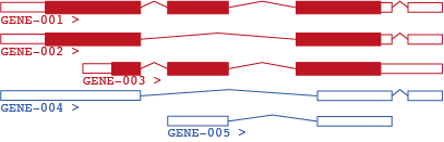
Figure 3.1: Transcript and intron-exon structure of a typical eukaryotic gene
Popular sources of human and mouse genome annotation are RefSeq, ENSEMBL, and GENCODE. RefSeq is the most conservative of the three, and tends to have the fewest annotated transcripts per gene. RefSeq transcript IDs start with NM_ or NR, e.g. NM_12345. ENSEMBL and GENCODE are very similar to each other and can be used interchangeably for our purposes. Gene names in these start with ENSG (for human) and ENSMUSG (for mouse); transcripts start with ENST and ENSMUST, respectively.
In addition to gene IDs, most genes also have a common name (“gene symbol”) assigned to them; e.g. human actin B will have ensembl gene ID ENSG00000075624 and symbol ACTB. Human gene names are regularly updated and defined by HGNC. Mouse gene names are decided by a similar consortium, MGI.
Current ENSEMBL/GENCODE annotation of the human genome contains approximately 60k genes, 20k of which are protein coding, and 237k transcripts. Most genes can be coarsely divided by type into protein coding genes, long noncoding RNAs, short noncoding RNAs, and pseudogenes. On a higher resolution, over 40 biotypes are defined. Gene biotype annotation also often changes between annotation versions (see below).
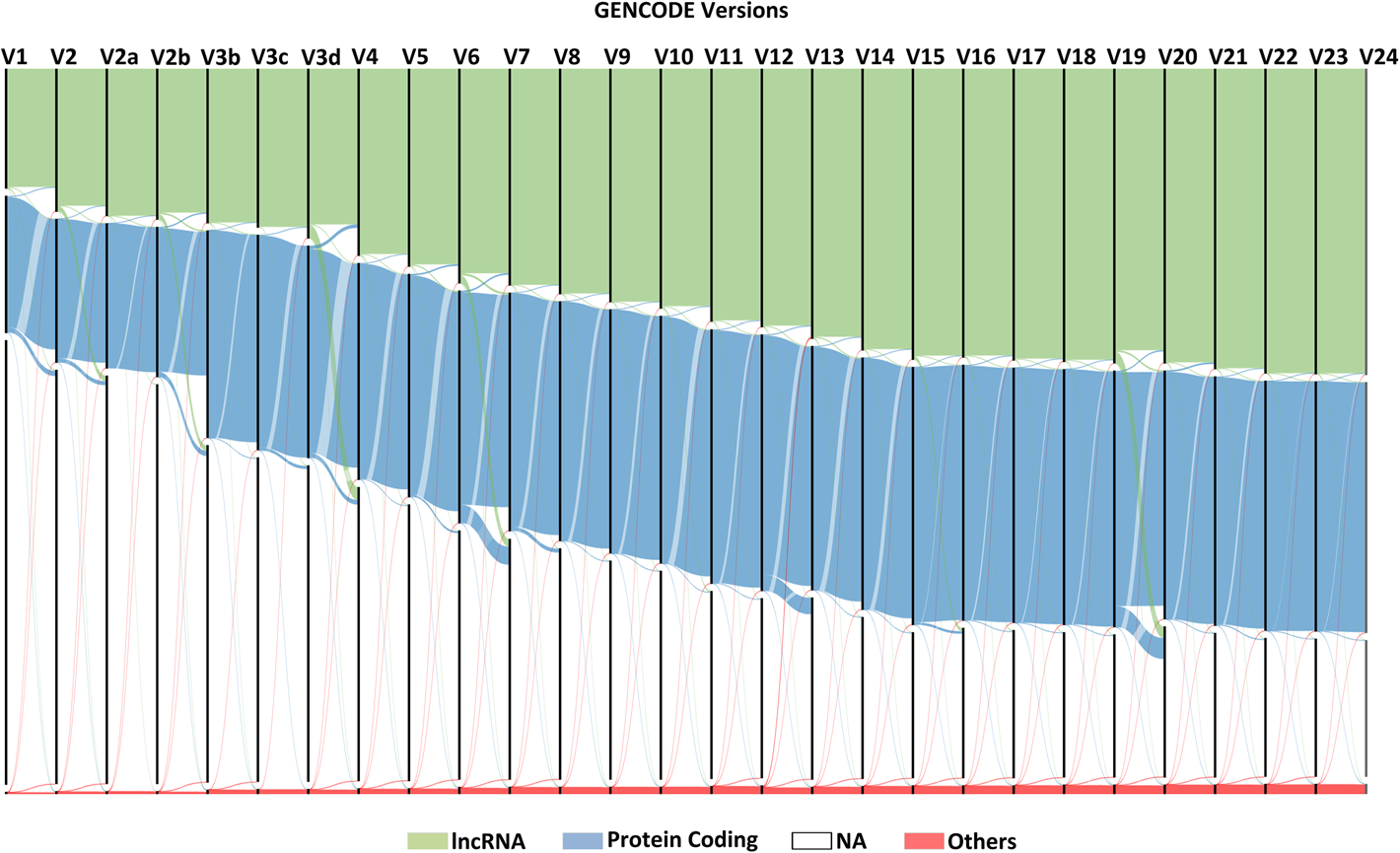
Figure 3.2: Sankey diagram of gene type changes in GENCODE versions
3.2 Processing of Bulk RNA-seq and Full-length scRNA-seq Data
Raw read processing of bulk RNA-seq is usually done in two steps: read alignment and read counting. Both steps contain important caveats which can strongly influence expression estimates for individual genes. Read alignment can be done against a genome or transcriptome reference. Because of widespread splicing in animal genomes, read alignment against a genome has to be done with a splice-aware aligner; two most popular modern tools are STAR and hisat2. Typical read coverage is shown in panel A below; note that read coverage is relatively uniform across both 3’ and 5’ ends of the given gene. Some reads perfectly align to more than 1 location; these reads are often referred to as multimappers. The ambiguity is much greater when aligning to transcriptome because many transcripts are very similar to each other (e.g. differ by only one exon); however, it is noticeable even on a gene level (panel B below).
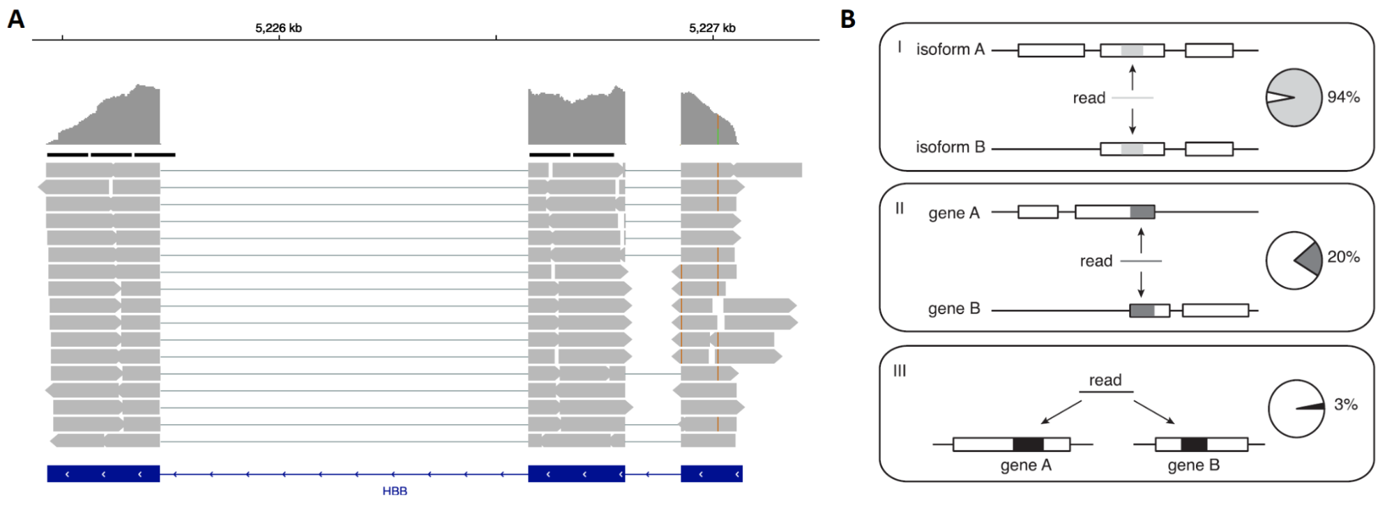
Figure 3.3: A: typical read coverage in a bulk RNA-seq or Smart-seq2 experiment; B: types of ambiguity that arise when reads are assigned to features
After alignment to the genome or transcriptome, read counts can be summarized on a gene or transcript level. In case of genome alignment, the simplest strategy is to count only reads mapping to a unique location (non-multimappers), and only overlapping one gene. This, however, inevitably creates a bias in gene expression estimates (Pachter, 2011). Somewhat more advanced strategy includes splitting read counts between features it aligns to (e.g. if a read aligns equally well to 3 paralogous genes, each paralog gets ⅓ of a count). Strand-specific RNA-seq reduces the ambiguity of read assignment in case of overlapping features located on opposite strands. An example of a program that efficiently implements all of the above-mentioned counting methods is featureCounts from the Subread package.
When transcriptome alignment is used, read assignment ambiguity is too great for simple counting. Thus, per-transcript and per-gene abundances are calculated using maximum likelihood abundance estimates using the Expectation-Maximization (EM) algorithm. This approach results in varying fractions of the read being assigned to features it maps to, and substantially reduces the bias related to multimappers. Reads (and read fractions) that are assigned to transcripts are then summarized on gene level. The most widely used and well-supported program implementing this strategy is RSEM. Generally speaking, this is the most accurate way of bulk RNA-seq quantification (Pachter, 2011).
An alternative to a conventional approach described above (alignment, then read quantification) is based on so-called pseudo-alignment methods. Two popular tools, kallisto and salmon, use very similar approaches:
- Split the reference transcriptome into k-mers and make a De Bruijn graph;
- Convert RNA-seq reads into k-mers;
- Use the k-mers to assign reads to a transcript or several transcripts (“equivalence class”);
- Summarize the resulting counts on a transcript or gene level.
Expectation-Maximization algorithm is used to find optimal distribution of reads that map to multiple transcripts. Both tools are extremely memory- and CPU-efficient, and quite accurate, especially for paired-end or long single-end reads. Pseudoalignment does not generate an alignment BAM file, so if visualization is needed (e.g. when using RNA-seq for transcript annotation) alignment should also be performed separately.
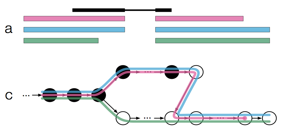
Figure 3.4: Pseudoalignment to transcriptome De Bruijn graph
Several things should be noted about bulk RNA-seq quantification. First, it is generally assumed that the number of sequenced cDNA fragments is proportional to the amount of RNA present in a cell. Thus when paired-end reads are used, each read pair is counted only once, as it stems from the same cDNA fragment. For well-annotated genomes like human and mouse it is very common to use single-end reads for RNA-seq. Second, PCR duplicates are usually ignored in bulk RNA-seq, and UMI use also does not confer substantial benefits. Several independent studies indicated that duplicate removal or UMI use do not noticeably increase the statistical power of bulk RNA-seq.
Finally, while many differential expression methods use raw read counts, it is conventional to use within-sample normalization when doing clustering, PCA, and other types of exploratory analysis. The most popular method of such normalization is conversion of raw reads to Transcripts per Million (TPM). The conversion accounts for two biases: 1) different samples are sequenced at different depth, not directly related to gene expression differences; 2) long genes are expected to generate more cDNA fragments than the short ones. Thus, for TPM calculation, raw read counts are first divided by the effective transcript length, which is defined as transcript length - cDNA fragment size + 1. After this, the resulting numbers are scaled linearly to add up to one million. Thus, the sum of all TPM values for a particular sample is always equal to (approximately) 1,000,000.
3.3 Read Alignment and Quantification in Droplet-based scRNA-seq Data
3.3.1 General Considerations
Single cell RNA-seq data differ from bulk RNA seq in a number of ways (see Introduction to single cell RNA-Seq chapter above). Most modern scRNA-seq technologies generate read sequences containing three key pieces of information:
- cDNA fragment that identifies the RNA transcript;
- Cell barcode (CB) that identifies the cell where the RNA was expressed;
- Unique Molecular Identifier (UMI) that allows to collapse reads that are PCR duplicates.
In contrast to bulk RNA-seq, scRNA-seq deals with a much smaller amount of RNA, and more PCR cycles are performed. Thus, UMI barcodes become very useful and are now widely accepted in scRNAseq. Library sequencing is often done with paired-end reads, with one read containing CB + UMI (read 1 in 10x Chromium), and the other containing actual transcript sequence (read 2 in 10x Chromium).
A classical scRNA-seq workflow contains four main steps:
- Mapping the cDNA fragments to a reference;
- Assigning reads to genes;
- Assigning reads to cells (cell barcode demultiplexing);
- Counting the number of unique RNA molecules (UMI deduplication).
The outcome of this procedure is a gene/cell count matrix, which is used as an estimate of the number of RNA molecules in each cell for each gene.
3.3.2 Read Mapping in Cell Ranger
Cell Ranger is the default tool for processing 10x Genomics Chromium scRNAseq data. It uses STAR aligner, which performs splicing-aware alignment of reads to the genome. After this, it uses the transcript annotation GTF to bucket the reads into exonic, intronic, and intergenic, and by whether the reads align (confidently) to the genome. A read is exonic if at least 50% of it intersects an exon, intronic if it is non-exonic and intersects an intron, and intergenic otherwise (shown below). Following the read type assignment, mapping quality adjustment is done: for reads that align to a single exonic locus but also align to 1 or more non-exonic loci, the exonic locus is prioritized and the read is considered to be confidently mapped to the exonic locus and given a maximum mapping quality score.
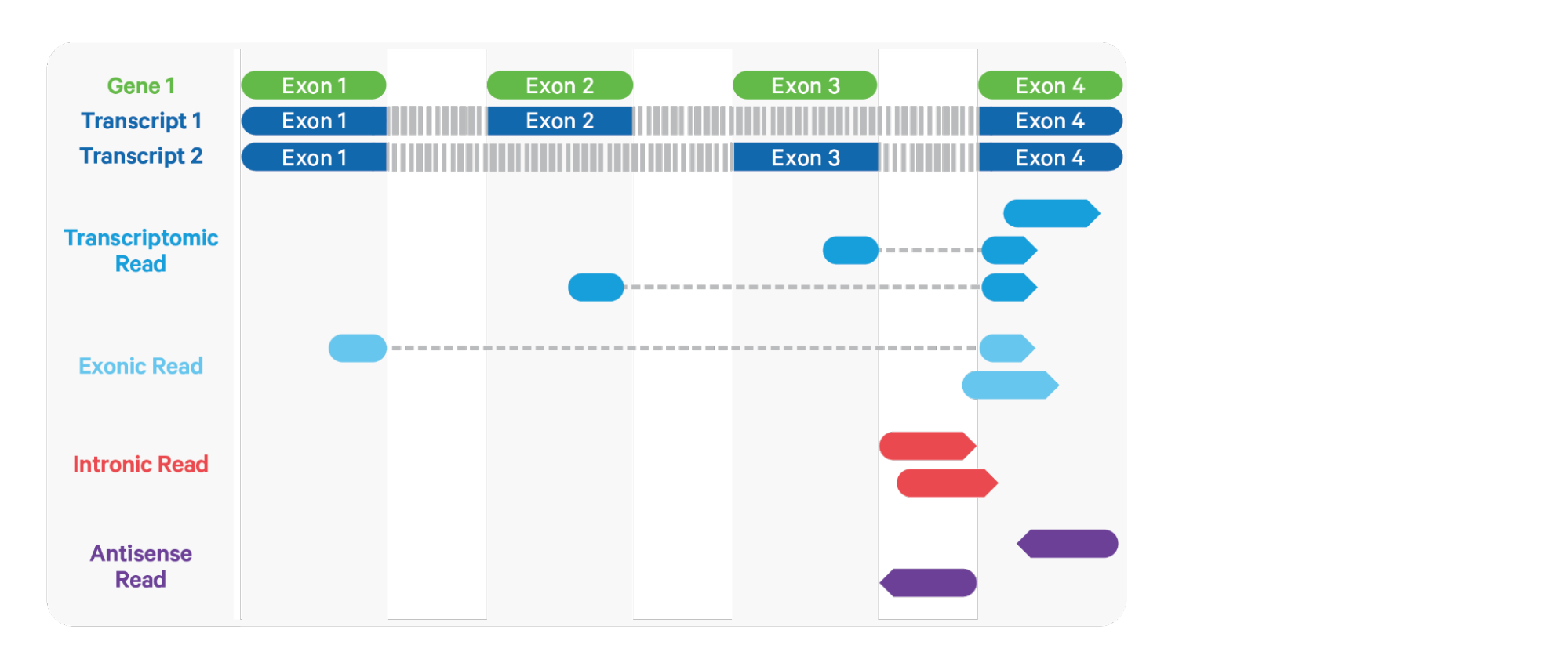
Figure 3.5: Classification of aligned reads in Cell Ranger
Cell Ranger further aligns exonic and intronic confidently mapped reads to annotated transcripts by examining their compatibility with the transcriptome. Reads are classified based on whether they are sense or antisense and based on whether they are exonic, intronic or whether their splicing pattern is compatible with transcript annotations associated with that gene. By default, reads that are transcriptomic (blue in the figure above) are carried forward to UMI counting.
When the input to the assay consists of nuclei, a high percentage of the reads comes from the unspliced transcripts and align to introns. In order to count these intronic reads, the “cellranger count” and “cellranger multi” pipelines can be run with the option include-introns. If this option is used, any reads that map in the sense orientation to a single gene - which include the reads labeled transcriptomic (blue), exonic (light blue), and intronic (red) in the diagram above - are carried forward to UMI counting. The include-introns option eliminates the need for a custom “pre-mRNA” reference that defines the entire gene body to be an exon.
Importantly, a read is considered uniquely mapping if it is compatible with only a single gene. Only uniquely mapping reads are carried forward to UMI counting; multimapping reads are discarded by Cell Ranger. In the Web Summary HTML output, the set of reads carried forward to UMI counting is referred to as “Reads mapped confidently to transcriptome.”
3.3.3 Cell Ranger Reference Preparation
Before we dive into the details of reference processing, it’s important to note how default Cell Ranger human and mouse references are prepared. Primary genome assembly versions (i.e. without the ALT loci) are used for the alignment in all versions. Annotation GTF files are filtered, using the scripts that could be found here. The following biotypes are retained: protein coding, long noncoding RNA, antisense, and all biotypes belonging to BCR/TCR (i.e. V/D/J) genes (note that older Cell Ranger reference versions do not include the latter). All pseudogenes and small noncoding RNAs are removed.
There are several versions of Cell Ranger reference that come pre-packaged with the software; 2020-A is the newest version of reference to date. All individual assembly and annotation combinations used by Cell Ranger previously are listed below. The unfiltered scRNAseq expression matrix generated using each reference is expected to contain the number of rows equal to the value in the “genes after filtering” column. Additionally, Cell Ranger also contains human + mouse combined reference, which is useful for experiments involving both human and mouse cells.
| Cell Ranger Reference | Species | Assembly/Annotation | Genes before filtering | Genes after filtering |
|---|---|---|---|---|
| 2020-A | human | GRCh38/GENCODE v32 | 60668 | 36601 |
| 2020-A | mouse | mm10/GENCODE vM23 | 55421 | 32285 |
| 3.0.0 | human | GRCh38/Ensembl 93 | 58395 | 33538 |
| 3.0.0 | human | hg19/Ensembl 87 | 57905 | 32738 |
| 3.0.0 | mouse | mm10/Ensembl 93 | 54232 | 31053 |
| 2.1.0 | mouse | mm10/Ensembl 84 | 47729 | 28692 |
| 1.2.0 | human | GRCh38/Ensembl 84 | 60675 | 33694 |
| 1.2.0 | human | hg19/Ensembl 82 | 57905 | 32738 |
| 1.2.0 | mouse | mm10/Ensembl 84 | 47729 | 27998 |
3.3.4 Chromium Versions and Cell Barcode Whitelists
Cellular barcode sequences are synthetic sequences attached to the beads that identify individual cells. The library of unique sequences is called a whitelist and depends on the Chromium library preparation kit version. The whitelist files are available from the Cell Ranger repository. There are three whitelists used for Chromium: 737K-april-2014_rc.txt, 737K-august-2016.txt, and 3M-february-2018.txt. CBs from the first list are 14 bp long, and two others are 16 bp. The table below provides cellular barcodes and UMI lengths, as well as appropriate whitelist files, for popular 10x single cell sequencing kits:
| Chemistry | CB, bp | UMI, bp | Whitelist file |
|---|---|---|---|
| 10x Chromium Single Cell 3’ v1 | 14 | 10 | 737K-april-2014_rc.txt |
| 10x Chromium Single Cell 3’ v2 | 16 | 10 | 737K-august-2016.txt |
| 10x Chromium Single Cell 3’ v3 | 16 | 12 | 3M-february-2018.txt |
| 10x Chromium Single Cell 3’ v3.1 (Next GEM) | 16 | 12 | 3M-february-2018.txt |
| 10x Chromium Single Cell 5’ v1.1 | 16 | 10 | 737K-august-2016.txt |
| 10x Chromium Single Cell 5’ v2 (Next GEM) | 16 | 10 | 737K-august-2016.txt |
| 10x Chromium Single Cell Multiome | 16 | 12 | 737K-arc-v1.txt |
Cell Ranger uses the following algorithm to correct putative barcode sequences against the whitelist :
- Count the observed frequency in the dataset of every barcode on the whitelist;
- For every observed barcode in the dataset that is not on the whitelist, find whitelist sequences that are 1-Hamming-distance away. For each such sequence:
- Compute the posterior probability that the observed barcode originated from the whitelist barcode with a sequencing error at the differing base (based on the base Q score);
- Replace the observed barcode with the whitelist barcode with the highest posterior probability that exceeds 0.975.
The corrected barcodes are used for all downstream analysis and output files. In the output BAM file, the original uncorrected barcode is encoded in the CR tag, and the corrected barcode sequence is encoded in the CB tag. Reads that are not able to be assigned a corrected barcode will not have a CB tag. In case you’re wondering why 3M-february-2018.txt file actually contains over 6 million unique sequences, the explanation can be found here.
3.3.5 UMI Counting
What is usually referred to as “UMI counting” consists of read counting followed by PCR duplicate collapsing based on UMI sequences. Before counting UMIs, Cell Ranger attempts to correct for sequencing errors in the UMI sequences. Reads that were confidently mapped to the transcriptome are placed into groups that share the same barcode, UMI, and gene annotation. If two groups of reads have the same barcode and gene, but their UMIs differ by a single base (i.e., are Hamming distance 1 apart), then one of the UMIs was likely introduced by a substitution error in sequencing. In this case, the UMI of the less-supported read group is corrected to the UMI with higher support.
Cell Ranger again groups the reads by barcode, UMI (possibly corrected), and gene annotation. If two or more groups of reads have the same barcode and UMI, but different gene annotations, the gene annotation with the most supporting reads is kept for UMI counting, and the other read groups are discarded. In case of a tie for maximal read support, all read groups are discarded, as the gene cannot be confidently assigned.
After these two filtering steps, each observed barcode, UMI, gene combination is recorded as a UMI count in the unfiltered feature-barcode (i.e. gene-cell) matrix. The number of reads supporting each counted UMI is also recorded in the molecule info file.
3.3.6 Cell Filtering
Unfiltered (“raw”) feature-barcode matrix contains many columns that are in fact empty droplets. Gene expression counts in these droplets are not zero due to technical noise, e.g. the presence of ambient RNA from broken cells. However, they can usually be distinguished from bona fide cells by the amount of RNA present. There are two algorithms implemented for this cell filtering in Cell Ranger, that we will refer to as “Cell Ranger 2.2” and “Cell Ranger 3.0” filtering.
The original algorithm (Cell Ranger 2.2) identified the first “knee point” in the “barcode count vs UMIs per barcode” plot. Cell Ranger 3.0 introduced an improved cell-calling algorithm that is better able to identify populations of low RNA content cells, especially when low RNA content cells are mixed into a population of high RNA content cells. For example, tumor samples often contain large tumor cells mixed with smaller tumor infiltrating lymphocytes (TIL) and researchers may be particularly interested in the TIL population. The new algorithm is based on the EmptyDrops method (Lun et al., 2018).
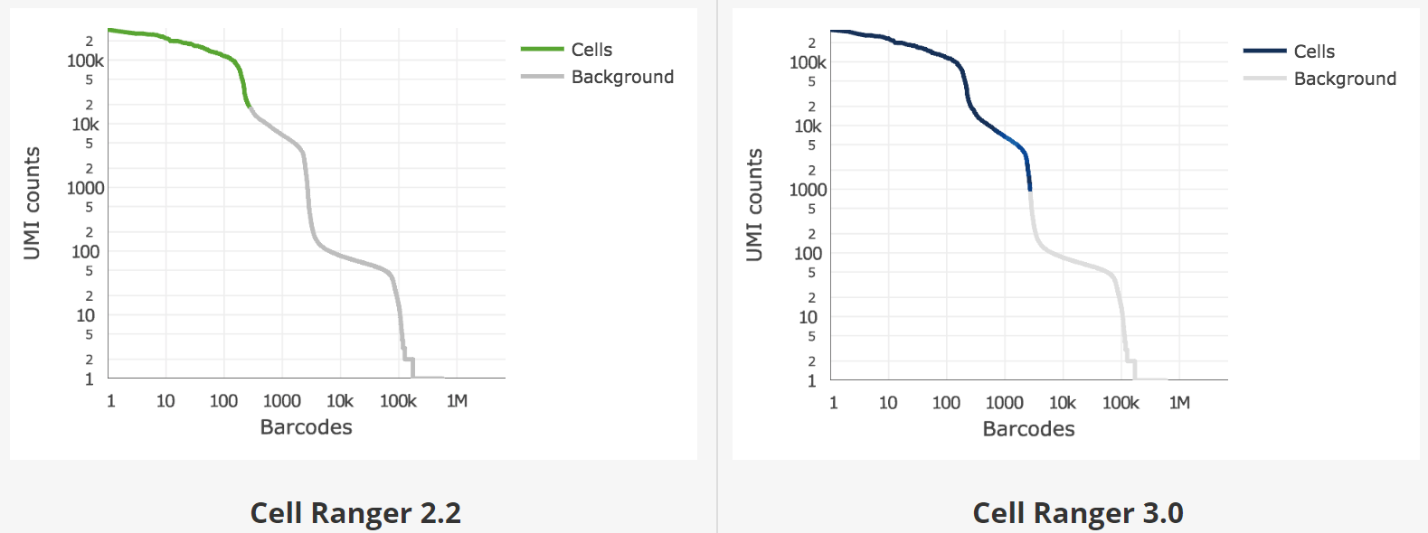
Figure 3.6: Knee plots and empty drop cutoffs identified by the Cell Ranger 2.2 and 3.0 filtering algorithms
3.3.7 Pseudoalignment-based Methods
Pseudoalignment (see above) can also be used to quickly quantify scRNA-seq datasets. Currently, there are two software suites that implement this approach: kallisto/BUStools, and Salmon/Alevin/Alevin-fry. In order to preserve the modular approach, both ecosystems introduced their own format that allows the storage of quantification results: kallisto/BUStools introduced the BUS (Barcode, UMI, and Set) file format (Melsted et al, 2019), while Alevin/Alevin-fry is using RAD format for the same purpose (Srivastava et al, 2019).
Both kallisto/BUStools and Alevin/Alevin-fry implement their own algorithms for cell barcode and UMI error correction and demultiplexing - for example, Alevin does not require (but can use) a cell barcode whitelist. However, the biggest difference from alignment-based methods stems from the lower accuracy of pseudoalignment, and the inclusion of multimapping reads.
kallisto/BUStools supports many sequencing technologies, including low-throughput ones like CEL-seq, CEL-seq2, and SMART-seq. The full list of supported experiments can be printed with kb --list. Alevin currently supports only the two most popular droplet based single-cell protocols, Drop-seq and 10x Chromium.
In general, kallisto/BUStools and Alevin are extremely efficient, allowing processing of human or mouse datasets with 2-4 Gb of RAM and at least an order of magnitude faster than Cell Ranger. Both tools also handle multimapping reads correctly, reducing the quantification bias for the affected genes. However, it has been noted in several publications that pseudoalignment-based methods falsely map reads from retained introns to the transcriptome (Melsted et al, 2021; Srivastava et al, 2020). It is well known that scRNA-seq experiments, and, in particular, single-nucleus RNA-seq can contain a very high percentage of transcripts with retained introns. This erroneous assignment makes hundreds of non-expressed genes look weakly expressed, which may substantially influence the downstream analysis, particularly marker selection (Kaminow et al, 2021). Thus, there is still a push to develop methods that would be at least as accurate and much faster than Cell Ranger.
3.4 STARsolo and Alevin-full-decoy: High Speed and High Accuracy
STARsolo is a standalone pipeline that is a part of STAR RNA-seq aligner mentioned in this chapter previously. It was developed with a goal to generate results that are very similar to Cell Ranger, while remaining computationally efficient. Normally, STARsolo is several times faster than Cell Ranger on the same dataset. STARsolo methods for UMI collapsing, cell barcode demultiplexing, and cell filtering are purposefully re-implementing the algorithms used by Cell Ranger. Starting from the STAR version 2.7.9a, STARsolo is also capable of quantifying multimapping read correctly, making it a very attractive option for fast and accurate scRNA-seq processing (Kaminow et al, 2021). Additional benefit of STARsolo is its flexible implementation of cellular barcode and UMI search: knowing a relative location within a read, and length of each sequence, it’s possible to process the data generated by most scRNA-seq approaches.
Alevin developers has also acknowledged the above-mentioned problem of intronic reads, developing a special solution which involved the use of so-called decoy sequences. In a recent STARsolo preprint, Alevin with full genome decoy has shown accuracy that is very similar to that of STARsolo or Cell Ranger (Kaminow et al, 2021).
3.5 Notes on Non-model Organisms
It is becoming increasingly popular to use single-cell RNA-seq for characterization of less known multicellular organisms, especially as a part of de novo genome assembly projects of key species. Two things are important to note here. First of all, a correctly assembled and well-annotated mitochondrial sequence is crucial, because mitochondrial reads constitute a substantial fraction of every scRNA-seq library and are widely used for experiment quality control (see Introduction to scRNA-seq). A recent effort has put together a compendium of carefully assembled mitochondrial sequences for many non-model vertebrates (Formenti et al, 2021). MITOS2 is a specialized server that can be used to automatically generate good quality mitochondrial annotations for metazoans.
Second, it is important to notice that most annotation methods for de novo sequenced genomes generate gene models that do not include UTR sequences. Both 3’ and 5’ scRNA-seq methods are heavily biased in their read distribution towards either end of the gene (figure below). Thus, using gene annotation that does not have UTR sequences will dramatically distort the results of quantification and analysis.
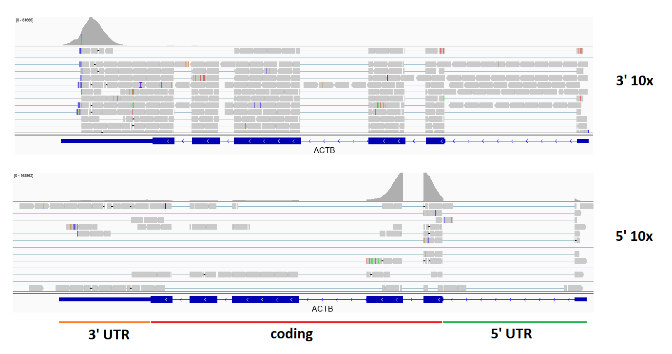
Figure 3.7: Typical read coverage in 3’ and 5’ 10x scRNA-seq experiments
3.6 Brief Summary and Processing Recommendations
Cell Ranger is the default software suite offered by 10x Genomics, and it remains the most widely used tool for read alignment and quantification. If you lack experience in bioinformatics, or have many other samples processed with Cell Ranger, stick with it. We would encourage you to use the latest Cell Ranger version, and the latest annotation files it comes with (see 3.3 above). At the same time, STARsolo and Alevin-full_decoy offer great computational speed-up and correct processing of multimappers, which reduces the quantification bias while retaining very high compatibility with Cell Ranger. They probably are the best option for users experienced with terminal tools. Finally, if you’re working with a poorly annotated genome, make sure your gene models include UTRs, and that you have a well-assembled and annotated mitochondrion.