2 Introduction to Single-Cell RNA-seq
QUESTIONS
- What is single-cell RNA-seq and how does it compare to bulk RNA-seq?
- What are some of the typical applications of scRNA-seq?
- How are samples typically prepared for scRNA-seq?
- What are the differences between some of the most popular protocols and what are their advantages and disadvantages?
- What experimental design choices should be considered in scRNA-seq?
- What are some of the challenges of scRNA-seq data compared to bulk data?
2.1 Overview of Single-Cell RNA-seq
RNA-seq allows profiling the transcripts in a sample in an efficient and cost-effective way. It was a major breakthrough in the late 00’s and has become ever more popular since, largely replacing other transcriptome-profiling technologies such as microarrays. Part of its success is due to the fact that RNA-seq allows for an unbiased sampling of all transcripts in a sample, rather than being limited to a pre-determined set of transcripts (as in microarrays or RT-qPCR).
Typically, RNA-seq has been used in samples composed of a mixture of cells, referred to as bulk RNA-seq, and has many applications. For example, it can be used to characterise expression signatures between tissues in healthy/diseased, wild-type/mutant or control/treated samples. Or in evolutionary studies, using comparative transcriptomics of tissue samples across different species [refs]. Besides its use in transcript quantification, it can also be used to find and annotate new genes, gene isoforms, and other transcripts, both in model and non-model organisms.
However, with bulk RNA-seq we can only estimate the average expression level for each gene across a population of cells, without regard for the heterogeneity in gene expression across individual cells of that sample. Therefore, it is insufficient for studying heterogeneous systems, e.g. early development studies or complex tissues such as the brain.
To overcome this limitation, new protocols were developed that allow applying RNA-seq at single-cell level (scRNA-seq), with its first publication in 2009 (Tang et al. 2009). This technology became more popular from around 2014 (ref), when new protocols and lower sequencing costs made it more accessible. Unlike with the bulk approach, with scRNA-seq we can estimate a distribution of expression levels for each gene across a population of cells.
This allows us to answer new biological questions where cell-specific changes in the transcriptome are important. For example discovering new or rare cell types, identifying differential cell composition between healthy/diseased tissues or understanding cell differentiation during development. One of the most iconic uses of this technology is in building gene atlases (see box below), which provide a comprehensive compendium of the cell diversity in organisms, with many applications in health as well as fundamental research.
Single-cell atlases
There are many projects trying to provide a comprehensive catalogue of cells in an organism. Here is a non-exhaustive list of some of these projects:
- Human Cell Atlas (H. sapiens)
- Tabula Muris (M. musculus)
- Fly Cell Atlas (D. melanogaster)
- Cell Atlas of Worm (C. elegans)
- Arabidopsis Root Atlas (A. thaliana)
scRNA-seq datasets range from hundreds to millions of cells per study, and increase in size every year. There are several different protocols available, both commercial and open access, each with its own advantages and disadvantages. We will discuss some of these aspects in the following sections.
)](figures/moores-law.png)
Figure 2.1: Moore’s law in single cell transcriptomics, showing an increase in the throughput of experiments from tens to millions of cells in just over a decade. (image taken from Svensson et al.)
2.2 Sample Preparation Protocols
Broadly speaking, a typical scRNA-seq protocol consists of the following steps (illustrated in the figure below):
- Tissue dissection and cell dissociating to obtain a suspension of cells.
- Optionally cells may be selected (e.g. based on membrane markers, fluorescent transgenes or staining dyes).
- Capture single cells into individual reaction containers (e.g. wells or oil droplets).
- Extracting the RNA from each cell.
- Reverse-transcribing the RNA to more stable cDNA.
- Amplifying the cDNA (either by in vitro transcription or by PCR).
- Preparing the sequencing library with adequate molecular adapters.
- Sequencing, usually with paired-end Illumina protocols.
- Processing the raw data to obtain a count matrix of genes-by-cells
- Carrying several downstream analysis (the focus of this course).
This course deals mostly with the last step of this workflow, but it is important to consider some of the steps that come before that, as they have an impact on the properties of the data we get.
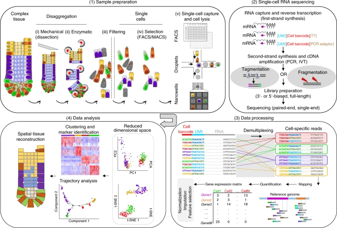
Schematic of a typical single-cell sequencing workflow. Abbreviations: IVT, in vitro transcription; PCR, polymerase chain reaction; UMI, unique molecular identifier. Image from Lafzi et al. 2018.
Single-nucleus RNA-seq
In tissues where cell dissociation is difficult or in frozen tissue samples, instead of isolating whole single cells it is possible to instead isolate single nuclei. Apart from the isolation step, the protocol to prepare single-nuclei sequencing libraries is similar to that of single-cell protocols. However, nuclear RNA usually contains a higher proportion of unprocessed RNA, with more of the sequenced transcripts containing introns. This aspect needs to be considered in the data processing steps, which we detail in the following chapter.
There are currently a wide diversity of protocols for preparing scRNA-seq data, each with its own strengths and weaknesses, which we will come to below. These methods can be categorized in different ways, but the two most important aspects are cell capture or isolation and transcript quantification.
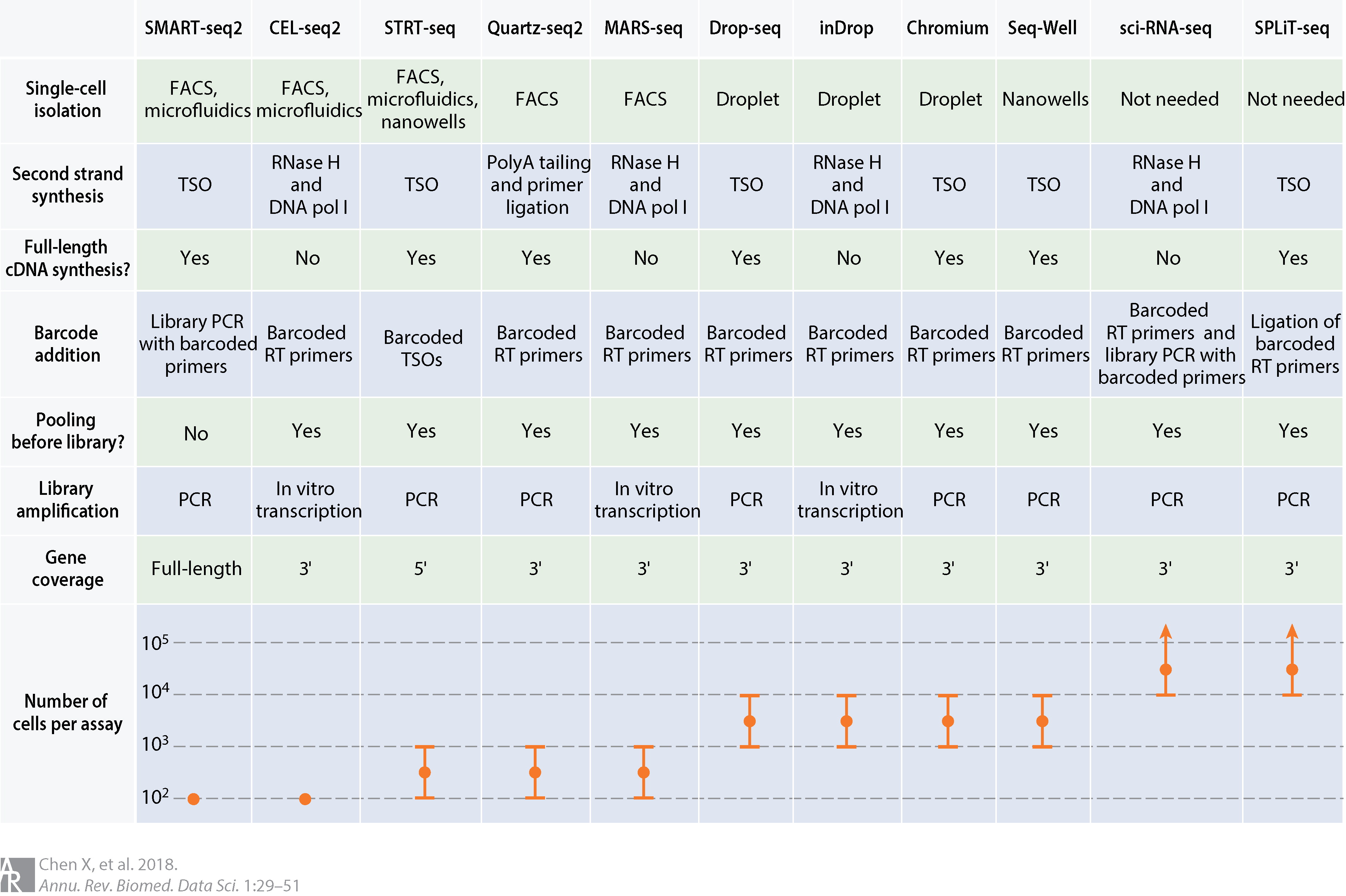
Comparison of common scRNA-seq protocols. Abbreviations: cDNA, complementary DNA; DNA pol I, DNA polymerase I; FACS, fluorescence-activated cell sorting; PCR, polymerase chain reaction; RNase H, ribonuclease H; RT, reverse transcription; TSO, template-switching oligonucleotide. (source: Chen, Teichman and Meyer, 2018)
2.3 Cell Capture
The strategy used for capturing cells determines the throughput of the experiment (i.e. how many cells we isolate), how the cells are selected prior to sequencing, as well as what kind of additional information besides transcript sequencing can be obtained. The three most widely used options are microtitre-plate-based, microfluidic-array-based and microfluidic-droplet-based methods.
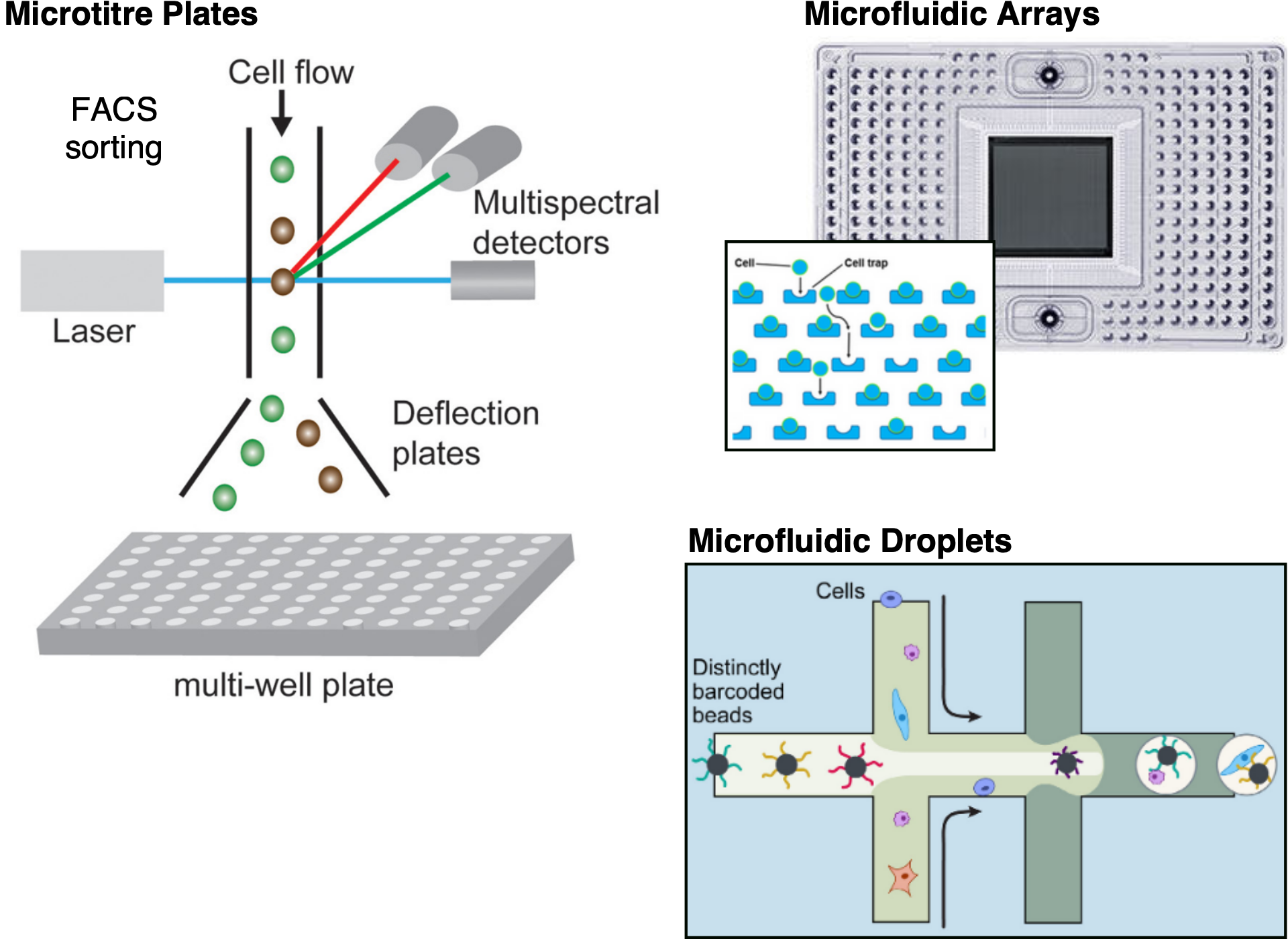
Single cell isolation methods.
Microtitre-plate methods rely on isolating cells into individual wells of the plate using, for example, pipetting, microdissection or fluorescent activated cell sorting (FACS). One advantage of well-based methods is that one can take pictures of the cells before library preparation, providing an additional data modality. For example one can identify and discard damaged cells or find wells containing doublets (wells with two or more cells). When using automatic FACS sorting, it is also possible to associate information such as cell size and the intensity of any used labels with the well coordinates, and therefore with individual cell indices in downstream analysis. The main drawback of these methods is that they are often low-throughput and the amount of work required per cell may be considerable.
Microfluidic-array platforms, such as Fluidigm’s C1, provide a more integrated system for capturing cells and for carrying out the reactions necessary for the library preparations. Thus, they provide a higher throughput than microtitre-plate-based methods. Typically, only around 10% of cells are captured in a microfluidic platform and thus they are not appropriate if one is dealing with rare cell-types or very small amounts of input. Care also has to be taken with the cell sizes captured by the arrays, as the nanowells are customised for particular sizes (this may therefore affect the unbiased sampling of cells in complex tissues). Moreover, the chip is relatively expensive, but since reactions can be carried out in a smaller volume, money can be saved on reagents.
Microfluidic-droplet methods offer the highest throughput and are the most popular method used nowadays. They work by encapsulating individual cells inside a nanoliter-sized oil droplet, together with a bead. The bead is loaded with enzymes and other components required to construct the library. In particular, each bead contains a unique barcode which is attached to all of the sequencing reads originating from that cell. Thus, all of the droplets can be pooled, sequenced together and the reads can subsequently be assigned to the cell of origin based on those barcodes. Droplet platforms have relatively cheap library preparation costs on the order of 0.05 USD/cell. Instead, sequencing costs often become the limiting factor and a typical experiment the coverage is low with only a few thousand different transcripts detected (Ziegenhain et al. 2017).
Fluorescence Activated Cell Sorting (FACS) can be used upstream of any of the capture methods, to select a sub-population of cells. A common way in which this is used is to stain the cells with a dye that distinguishes between live and dead cells (e.g. due to membrane rupture), thus enriching the cell suspension with viable cells.
2.4 Transcript Quantification
There are two types of transcript quantification: full-length and tag-based. Full-length protocols try to achieve a uniform read coverage across the whole transcript, whereas tag-based protocols only capture either the 5’ or 3’ ends. The choice of quantification method has important implications for what types of analyses the data can be used for.
Preparing full-length libraries for single-cell is essentially identical to what is done in bulk RNA-seq (Figure below), and is restricted to plate-based protocols such as SMART-seq2. Although in theory full-length protocols should provide an even coverage of transcripts, there can sometimes be biases in the coverage across the gene body (illustrated below). Full-length protocols also allow the detection of splice variants, which is very difficult to do with other protocols.
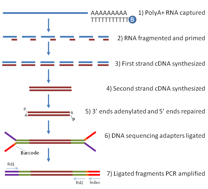
Full-length RNA library preparation for Illumina sequencing. Samples are enriched for RNA containing a poly(A) tail, which avoids sequencing rRNA (at the cost of also missing other non-coding RNAs). The RNA is then fragmented and reverse-transcribed to more stable cDNA, Illumina adapters ligated to each molecule and finally PCR-amplified. In the case of single-cell RNA-seq, adapters with well-specific barcodes are used, allowing to identify sequencing reads belonging to individual cells. Image source []. (source)
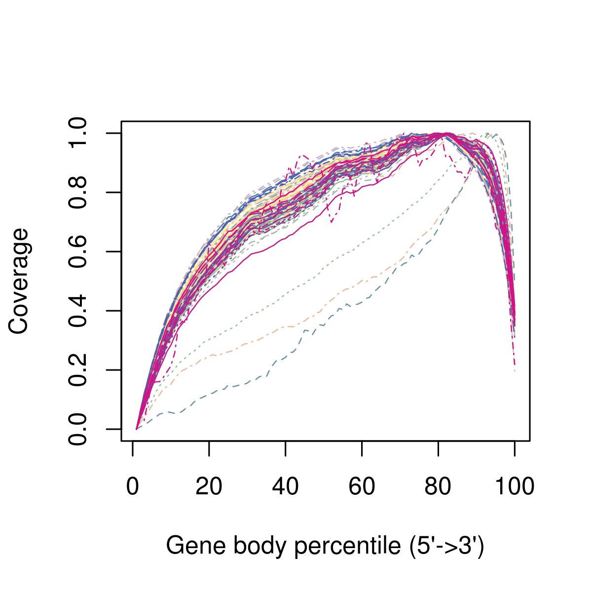
Figure 2.2: Example of 3’ bias in the gene body coverage, after aligning the sequencing reads to the transcriptome. Each line represents the average coverage across all the genes in a cell. In this example, in addition to the 3’ bias across all cells, there are three cells that look like outliers relative to the rest and should be removed from downstream analysis. These may be cells where RNA quality was poorer, e.g. due to degradation.
With tag-based protocols, only one of the ends (3’ or 5’) of the transcript is sequenced. The main advantage of tag-based protocols is that they can be combined with unique molecular identifiers (UMIs), which can help improve the accuracy of transcript quantification. The reason for this improvement has to do with the PCR amplification step during library preparation, which creates several duplicate copies of each molecule. Because this amplification is exponential, molecules may be unfairly represented in the final library, leading to over-estimation of their expression due to these PCR duplicates. To address this problem, cell barcodes are uniquely tagged with a random nucleotide sequence, the UMI, which is therefore unique to a single molecule. This UMI is part of the sequencing read and can then be computationally taken into account when quantifying the transcript’s abundance. Most current scRNA-seq protocols are tag-based, including the popular droplet-based 10x Chromium protocol, illustrated in the figure below. One disadvantage of tag-based protocols is that, being restricted to one end of the transcript only, it reduces our ability to unambiguously align reads to a transcript, as well as making it difficult to distinguish different isoforms (Archer et al. 2016).
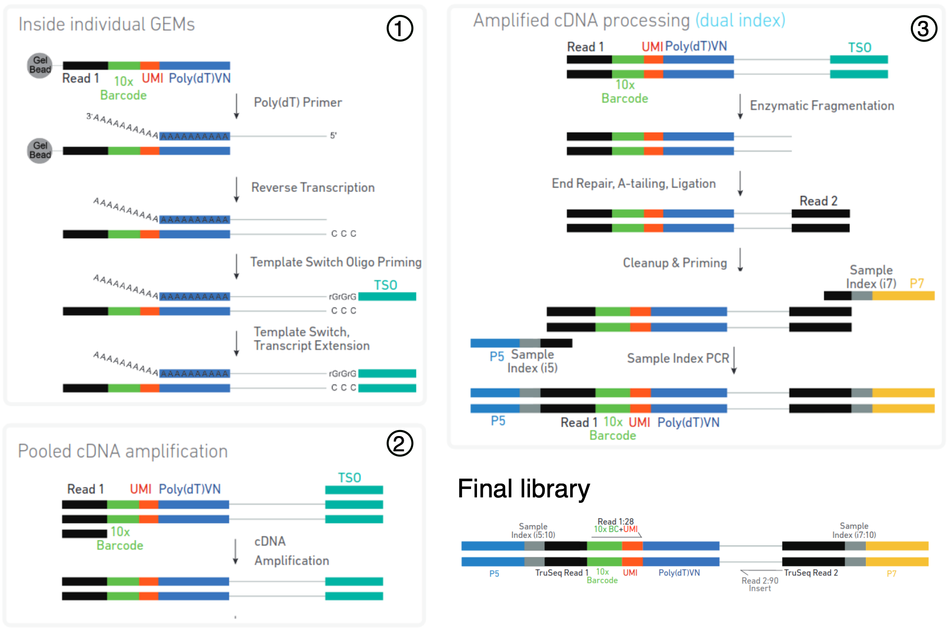
Protocol overview of 3’ libraries using the 10X Chromium protocol. Cells are captured in individual oil droplets containing a bead (called GEMs). An individual bead contains adapters with a common barcode, but diverse and distinct Unique Molecular Identifier (UMI) sequences. A poly(dT) primer is used to reverse-transcribe mRNA with poly-A tails into cDNA. The GEMs are then broken and the pooled cDNA (from all barcoded cells) is amplified by PCR. Finally, the cDNA is fragmented and another Illumina adapter is ligated at the other end of the molecule. The final library is composed of a read containing the cell-specific barcode (used to identify reads from different cells) and a molecule-specific UMI (used to quantify a gene’s expression), while the second read contains sequence from the actual cDNA molecule and can be used to align it to a reference transcriptome. (source: Chromium Next GEMSingle Cell 3ʹ User Guide)
5’ or 3’?
The difference between 5’ and 3’ tag-based protocols is which end of the transcript is sequenced. Although 3’ protocols are more commonly used, many protocols now allow sequencing from either end (e.g. 10x Chromium supports both). The advantage of 5’-end sequencing is that we obtain information about the transcription start site (TSS), which allows to explore whether there is differential TSS usage across cells.
2.5 Experimental Design
Several considerations need to be taken into account when performing scRNA-seq experiments. Factors such as the cost per cell, how many cells one needs, or how much to sequence each cell, may all influence our choice of protocol. On the other hand, care has to be taken to avoid biases due to batches being processed at different times and a lack of adequate replication may also constrain the types of analysis that can be done and therefore limit our ability to answer some questions of interest.
2.5.1 What Protocol Should I Choose?
The most suitable platform depends on the biological question at hand. For example, if one is interested in characterizing the composition of a heterogeneous tissue, then a droplet-based method is more appropriate, as it allows a very large number of cells to be captured in a mostly unbiased manner. On the other hand, if one is interested in characterizing a specific cell-population for which there is a known surface marker, then it is probably best to enrich using FACS and then sequence a smaller number of cells at higher sequencing depth.
Clearly, full-length transcript quantification will be more appropriate if one is interested in studying different isoforms, since tagged protocols are much more limited in this regard. By contrast, UMIs can only be used with tagged protocols and they can improve gene-level quantification.
If one is interested in rare cell types (for which known markers are not available), then more cells need to be sequenced, which will increase the cost of the experiment. A useful tool to estimate how many cells to sequence has been developed by the Satija Lab: https://satijalab.org/howmanycells/.
Another way to decide on which method to use, is to rely on studies dedicated to comparing different protocols. These studies focus on issues such as sensitivity (how many genes are detected per cell), their accuracy (e.g. compared to bulk RNA-seq) and in their ability to recover all cell types present in a sample (tested on commercially available cell mixtures). For example, a study by Ding et al. 2020 illustrates how low-throughput methods have higher sensitivity compared to high-throughput methods, such as 10x Chromium (Figure below). On the other hand, low-throughput methods did not capture some of the rarer cell types in their samples, leading to an incomplete characterisation of the cell population.
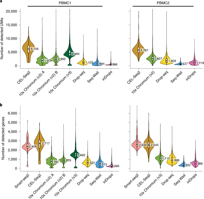
Transcript detection sensitivity of different methods in a commercial mixture of peripheral blood mononuclear cells (PBMCs). The figure is taken from Ding et al. and shows a) the number of distinct UMIs detected per cell (for methods using tag-based transcript quantification) and b) the number of detected genes per cell across methods. Results from two experimental replicates are shown.
Another study by Ziegenhain et al. (Ziegenhain et al. 2017) compared five different protocols on the same sample of mouse embryonic stem cells (mESCs), reaching similar conclusions. And finally, a study by Svensson et al. (Svensson et al. 2017) used synthetic transcripts (spike-ins) with known concentrations to measure the accuracy and sensitivity of different protocols. Comparing a wide range of studies, they also reported substantial differences between the protocols (Figure below).
, comparing different protocols in relation to their a) accuracy (measured as the Pearson's correlation with bulk RNA-seq data) and b) sensitivity (number of detected molecules).](figures/svenssonTeichmannFig2.png)
Figure 2.3: Figure from Svensson et al., comparing different protocols in relation to their a) accuracy (measured as the Pearson’s correlation with bulk RNA-seq data) and b) sensitivity (number of detected molecules).
As protocols are developed and improved, and new computational methods for quantifying the technical noise emerge, it is likely that future studies will help us gain further insights regarding the strengths of the different methods. These comparative studies are helpful not only to decide on which protocol to use, but also for developing new methods as the benchmarking makes it possible to determine what strategies are the most useful ones.
Besides differences in throughput and sensitivity between protocols, cost may also be a deciding factor when planning a scRNA-seq experiment. It is difficult to precisely estimate how much an experiment will cost, although we point to this tool from the Satija Lab as a starting point: https://satijalab.org/costpercell/. For example, some droplet-based protocols such as Drop-seq are cheaper than the commercial alternatives such as 10x Chromium. However, they require the labs to be equipped to prepare the libraries, as well as trained staff and dedicated time (costing salary money).
Methods such as cell hashing (Stoeckius et al.) may further reduce the costs of sequencing using current platforms. This method in particular consists of attaching oligo-tags to cell membranes, allowing more cells from multiple samples to be loaded per experiment, which can later be demultiplexed during the analysis.
2.5.2 Data Challenges
The main difference between bulk and single cell RNA-seq is that each sequencing library represents a single cell, instead of a population of cells. Therefore, there is no way to have “biological replicates” at a single-cell level: each cell is unique and impossible to replicate. Instead, cells can be clustered by their similarity, and comparisons can then be done across groups of similar cells (as we shall see later in the course).
Another big challenge in single-cell RNA-seq is that we have a very low amount of starting material per cell. This results in very sparse data, where most of the genes remain undetected and so our data contains many zeros. These may either be due to the gene not being expressed in the cell (a “real” zero) or the gene was expressed but we were unable to detect it (a “dropout”). This leads to cell-to-cell variation that is not always biological but rather due to technical issues caused by uneven PCR amplification across cells and gene “dropouts” (where a gene is detected in one cell but absent from another (Kharchenko, Silberstein, and Scadden 2014)). Improving the transcript capture efficiency and reducing the amplification bias are solutions for these problems and still active areas of technical research. However, as we shall see in this course, it is possible to alleviate some of these issues through proper data normalisation.
Another important aspect to take into account are batch effects. These can be observed even when sequencing the same material using different technologies (figure below), and if not properly normalised, can lead to incorrect conclusions.
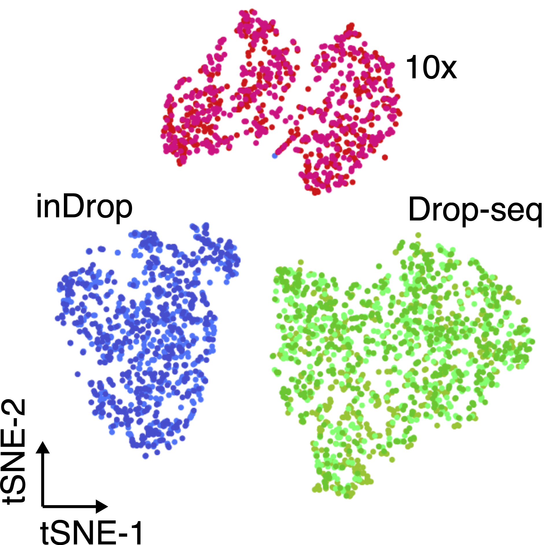
The same cell population was sequenced with three different single-cell protocols (colours). Adapted from Zhang et al..
The processing of samples should also be done in a manner that avoids confounding between experimentally controlled variables (such as a treatment, a genotype or a disease state) and the time when the samples are prepared and sequenced. For example, if planning an experiment to compare healthy and diseased tissues from 10 patients each, if only 10 samples can be processed per day, it is best to do 5 healthy + 5 diseased together each day, rather than prepare all healthy samples one day and all diseased samples in another (figure). Another consideration is to ensure that there is replication of tissue samples. For example, when collecting tissue from an organ, it may be a good idea to take multiple samples from different parts of the organ. Or consider the time of day when samples/replicates are collected (due to possible circadian changes in gene expression). In summary, all the common best practices in experimental design should be taken into account when performing scRNA-seq.
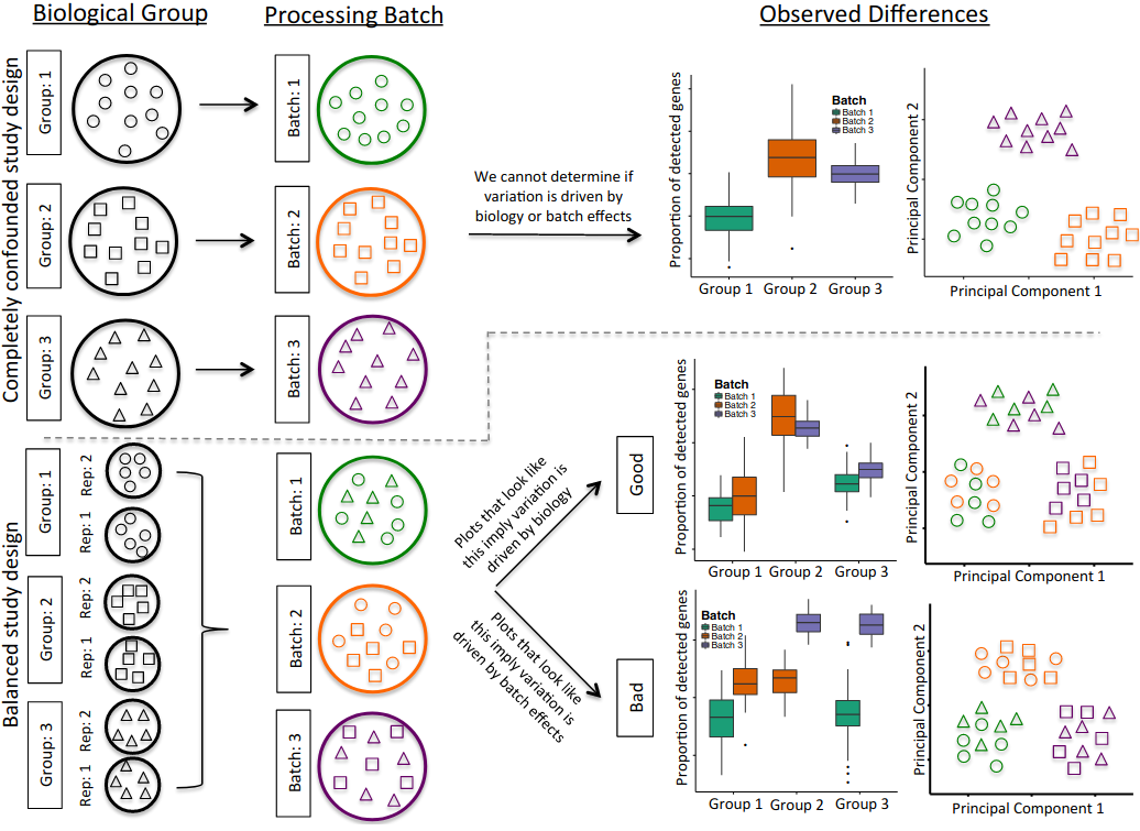
Illustration of a confounded (top panels) and balanced (bottom panels) designs. Shapes denote different sample types (e.g. tissues or patients) and colours processing batches. In the confounded design it’s impossible to disentangle biological variation from variation due to the processing batch. In the balanced design, by using tissue replicates and mixing them across batches, it is possible to distinguish between biological and batch-related variation. Figure from Hicks et al..
2.6 Summary
KEY POINTS
- scRNA-seq is ideally suited to study heterogeneous populations of cells. For example to identify the types of cells that compose a tissue, define “transcriptional fingerprints” for different cell types, study cell differentiation, explore changes in cell composition due to disease or environmental factors, amongst others.
- A typical sample preparation workflow consists of isolating single cells (or nuclei), converting the RNA into cDNA, preparing a sequencing library (Illumina) and sequencing.
- Many single-cell protocols have been developed, some openly available, others provided commercially. These mainly differ in their throughput (how many cells are captured per experiment), the type of quantification (full-length or tag-based) and also cost.
- SMART-seq2 is a popular low-throughput method, providing full-length transcript quantification. It is ideally suited for studying a smaller group of cells in greater detail (e.g. differential isoform usage, characterisation of lowly-expressed transcripts).
- 10x Chromium is a popular high-throughput method, using UMIs for transcript quantification (from either 3’ or 5’ ends). It is ideally suited to study highly heterogeneous tissues and sample large populations of cells at scale.
- When planning an experiment, care should be taken to avoid confounding due to batch effects as well as ensuring an adequate level of replication to address questions of interest.